Minimalist CNN for Medical Imaging Classiﬁcation with Small Dataset:

Does Size Really Matter and How?

Marie

Economid

1,2 a

and Pascal Desbarats

2 b

GE Healthcare, F-78530 Buc, France

Univ. Bordeaux, CNRS, Bordeaux INP, LaBRI, UMR 5800, F-33400 Talence, France

Keywords:

Deep Learning, Medical Imaging, MRI, Classiﬁcation, Convolutional Neural Network.

Abstract:

Deep learning has become a key method in computer vision, and has seen an increase in the size of both the

networks used and the databases. However, its application in medical imaging faces limitations due to the size

of datasets, especially for larger networks. This article aims to answer two questions: How can we design a

simple model without compromising classiﬁcation performance, making training more efﬁcient? And, how

much data is needed for our network to learn effectively? The results show that we can ﬁnd a minimalist

CNN adapted to a dataset that gives results comparable to larger architectures. The minimalist CNN does not

have a ﬁxed architecture. Its architecture varies according to the dataset and various criteria such as overall

performance, training stability, and visual interpretation of network predictions. We hope this work can serve

as inspiration for others concerned with these challenges.

1 INTRODUCTION

Last past years, Deep Learning (DL) methods demon-

strated high performances in computer vision tasks

like classiﬁcation, detection, or segmentation. Classi-

ﬁcation challenges on large datasets like MNIST (Le-

Cun et al., 2010), ImageNet (Fei-Fei et al., 2009) or

CIFAR10- CIFAR100 (Krizhevsky et al., 2009) have

driven the development of powerful neural networks

such as ResNet (He et al., 2016), VGG (Simonyan and

Zisserman, 2014), and AlexNet (Krizhevsky et al.,

2012). However, as the network size and complexity

increased, the need for larger datasets increased too.

In medical imaging, DL methods demonstrated

high performance in various applications like knee

abnormalities classiﬁcation and detection (Rizk et al.,

2021). However, medical datasets frequently lack

sufﬁcient volume compared to the architectures em-

ployed. Medical imaging dataset size is limited be-

cause of the complex process of collecting data en-

suring patient’s rights and the fastidious and time-

consuming annotation process. Confronted with such

small, often imbalanced datasets (Gao et al., 2020),

common strategies rely on data augmentation meth-

ods, like MRNet work (Bien et al., 2018) using ro-

https://orcid.org/0009-0001-3576-1526

https://orcid.org/0000-0003-4267-492X

tations or horizontal ﬂips. Additionally, a common

practice often involves pre-training models on non-

medical images (Kim et al., 2022). This introduces

irrelevant features and unnecessary parameters, lead-

ing to high computational costs.

An alternative approach involves designing more

suitable networks (Zavalsız et al., 2023), (Albelwi and

Mahmood, 2017). For instance, the framework pro-

posed by (Cao, 2015) relies on deconvolution for fea-

ture visualization and correlation coefﬁcient calcula-

tion for architecture optimization. Another work by

(Wasay and Idreos, 2020) introduces a design frame-

work centered on controlling the number of param-

eters in the network, along with a thorough analysis

of numerous parameters. These works offer valuable

insights into CNN design. However, they may not

necessarily address adaptation to a small dataset and

limited computational resources.

In this study, we aim to provide a methodology

to design the smallest possible Convolutional Neural

Network (CNN) adapted to a speciﬁc dataset while

maintaining accuracy comparable to more complex

CNNs, guided by the comprehension of learned fea-

tures.

This paper presents a preliminary study on the

minimalist CNN design based on preliminary results

on MRI classiﬁcation tasks and a comparison between

different architectures. In the ﬁrst step, a way of de-

Économidès, M. and Desbarats, P.

Minimalist CNN for Medical Imaging Classiﬁcation with Small Dataset: Does Size Really Matter and How?.

DOI: 10.5220/0012452700003660

Paper published under CC license (CC BY-NC-ND 4.0)

In Proceedings of the 19th International Joint Conference on Computer Vision, Imaging and Computer Graphics Theory and Applications (VISIGRAPP 2024) - Volume 2: VISAPP, pages

755-762

ISBN: 978-989-758-679-8; ISSN: 2184-4321

755

signing a minimalist CNN adapted to the dataset size

is introduced. Secondly, we present the dataset and

training parameters. Then, we focus on the compar-

ison between different architectures using different

criteria, especially comprehension of learned features

along with a discussion.

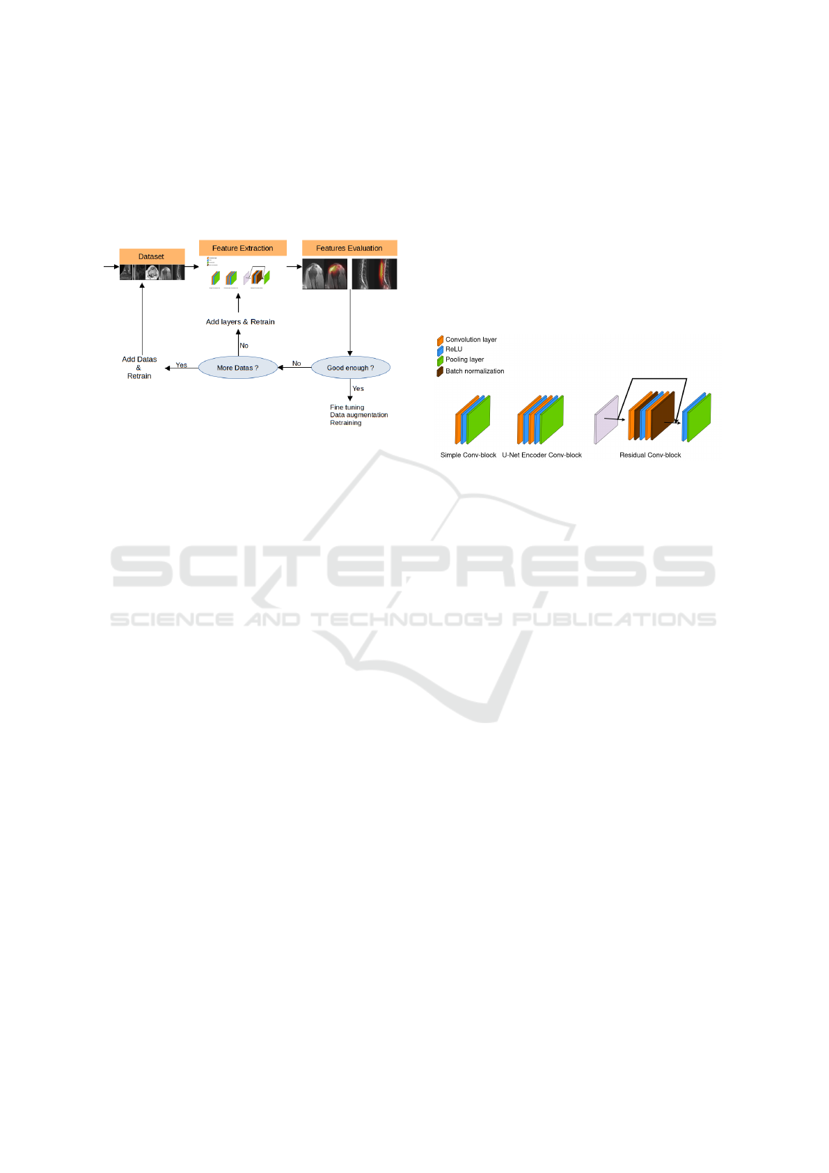
Figure 1: Illustration of the process of designing a minimal-

ist CNN.

2 METHOD

A Convolutional Neural Network (CNN) is composed

of a feature extractor and classiﬁer. Classical met-

rics will be employed for performance evaluation dur-

ing and after training. Visual explanations, specif-

ically GradCam, will provide a visual interpretation

of activations. Depending on the outcomes of previ-

ous training iterations, the model’s architecture can

be adjusted and enhanced by incorporating additional

conv-blocks.

2.1 Design Architecture

We design our minimalist CNN using convolutional

blocks (conv-blocks) for feature extraction and a clas-

siﬁer for ﬁnal predictions. This minimalist CNN aims

to be as small and lightweight as possible while per-

forming at least as well as larger models found in the

literature.

Design of Features Extractor. The features extrac-

tor is composed of conv-blocks. A convolutional

block in deep learning is a fundamental unit com-

prising convolutional layers, activation functions, op-

tional pooling, and normalization operations. It al-

lows feature extraction and processing at different

levels of abstraction, enabling convolutional neural

networks to learn hierarchical representations of vi-

sual information.

The ﬁrst layers allow for the extraction of high-

level features, corresponding to the global character-

istics of the image, while the deeper layers, known as

low-level layers, extract more speciﬁc features of the

image. This implies that a minimum number of con-

volutional layers is necessary to construct our model.

Figure 2 illustrates the different conv-block that

will serve to design a minimalist CNN and compare

it to bigger architectures. We take inspiration from

well-known models like LeNet5 (LeCun et al., 1998),

U-Net (Ronneberger et al., 2015) and ResNet (He

et al., 2016).

Figure 2: Illustration of different conv-blocks.

The ﬁrst conv-block is inspired by the LeNet5 ar-

chitecture. This CNN architecture was one of the ﬁrst

to demonstrate its effectiveness in classifying small

images and simple tasks such as digit recognition. In

a LeNet5 network, there are three convolutional lay-

ers followed by a tanh activation function, with two

of them followed by a pooling layer. We use this

architecture as a reference for the minimum number

of convolutional layers needed for feature extraction.

We deﬁne a simple conv-block as a convolutional

layer followed by an activation function and a pooling

layer. Based on this simple conv-block, we design a

feature extractor composed of 4 simple conv-blocks.

For clarity in the paper, we decide to refer to this net-

work as miniCNN.

The second illustrated conv-block is based on the

U-Net architecture, renowned for its superior perfor-

mance and precise predictions, even when working

with small datasets. Shaped like a ’U’, U-Net com-

prises an encoder that captures the contextual infor-

mation of the image, a decoder for accurate localiza-

tion and information expansion to restore the initial

image size, and a bottleneck connecting the encoder

and decoder. While its primary application is in seg-

mentation tasks, a closer examination of the encoder

component is interesting. A conv-block consists of

two consecutive convolutional layers, each followed

by a ReLU activation function, and concludes with a

pooling layer. Based on this conv-block, we design

a feature extractor composed of 5 conv-blocks. As it

refers to the encoder part of U-Net, we decide to refer

to this network as UEnc.

VISAPP 2024 - 19th International Conference on Computer Vision Theory and Applications

756

In related work by RadImageNet (Mei et al.,

2022), various well-known CNN architectures were

explored including the ResNet architecture. The ef-

fectiveness of this model to train very deep networks

has made it a popular choice across many applica-

tions. As our minimalist CNN aims to approach or

match the performance of larger networks with lim-

ited data, we decide to include this architecture in our

tests.

ResNet’s strength lies in its use of residual conv-

blocks and skip connections. It allows more direct

ﬂow of gradients and mitigates the Vanishing Gradi-

ent Problem. Moreover, it improves training speed

and convergence compared to different architectures.

ResNet also enables the training of larger models that

improve feature representation. However, it’s impor-

tant to note that this approach may increase com-

plexity and require more computational resources. It

may also be more sensitive to overﬁtting with smaller

datasets and interpretation of learned features can be

more difﬁcult. That is the reason why two versions

of ResNet will be trained: ResNet18 (RN18) and

ResNet50 (RN50).

Classiﬁer. After the feature extraction process, the

classiﬁer takes the extracted features as input and uti-

lizes them to assign labels and make predictions. The

classiﬁer is composed of one or more fully connected

layers, also known as dense layers. In addition to

the fully connected layers, an activation function like

softmax for multi-class classiﬁcation can be used to

convert outputs into probability scores for each class

and the highest probability corresponds to the pre-

dicted class. The classiﬁer architecture complexity

depends on the task and data. To improve perfor-

mance and generalization additional layers such as

dropout or normalization can be used with one or sev-

eral dense layers.

Considering the ResNet classiﬁer is composed of

1 Fully Connected layer followed by softmax, our

minimalist CNN classiﬁer will adopt the same struc-

ture.

Commonly used Cross Entropy loss function for

classiﬁcation tasks is given to measure model perfor-

mance.

2.2 Model Explanation

Obtaining a deeper understanding of our model’s

learning process is crucial for validating our mini-

malist CNN to ensure high precision and extraction

of meaningful features. To achieve this, we focus on

the Gradient Class Activation Mapping (Grad-CAM)

technique (Selvaraju et al., 2017). Additionally, we

enhance this visual interpretation of prediction by us-

ing a quantitative quality score for GradCam evalua-

tion.

Visual Explaination. Grad-CAM provides a visu-

alization that allows for the interpretation of CNN

predictions by indicating which parts of an image

have contributed the most to the classiﬁcation of an

image and the prediction of a speciﬁc class. Gradi-

ents at the output of a convolutional layer are com-

puted for a speciﬁc class. They are then weighted to

generate a heat map to highlight the most activated ar-

eas of the image. Multiple GradCAM methods have

been deployed. We choose to use ablationCAM (Ra-

maswamy et al., 2020), an improved version of clas-

sical GradCAM.

3 EXPERIMENTAL SETUP

We apply our method to a medical imaging problem,

speciﬁcally focusing on the classiﬁcation of osteoar-

ticular MRI. This section presents the dataset used,

training parameters, and details about the equipment

employed.

3.1 Dataset

In medical imaging, datasets are typically small and

imbalanced. Here, we choose to design a minimalist

model for osteoarticular MRI classiﬁcation, speciﬁ-

cally focusing on structure classiﬁcation. A typical

dataset consists of around 55 examinations. An ex-

amination is a series of images acquired in a speciﬁc

orientation, averaging about 32 images per series, to-

taling approximately 1760 images. For a given model,

training is conducted by varying the amount of data

without data augmentation. Our goal is to determine

if we can ﬁnd an architecture that is large enough

to achieve performance comparable to datasets with

thousands of images with this amount of data, yet as

small as possible to reduce training time and compu-

tational costs.

RadImageNet. Dataset (Mei et al., 2022) consists

of over a million images from various acquisitions,

modalities, and anatomical structures. From this

dataset, we choose to extract MRI osteoarticular data

which corresponds to 5 classes: Ankle, Hip, Knee,

Shoulder, and Spine.

Sub Datasets. To create the training, validation,

and test datasets, we initially split the dataset with a

Minimalist CNN for Medical Imaging Classiﬁcation with Small Dataset: Does Size Really Matter and How?

757

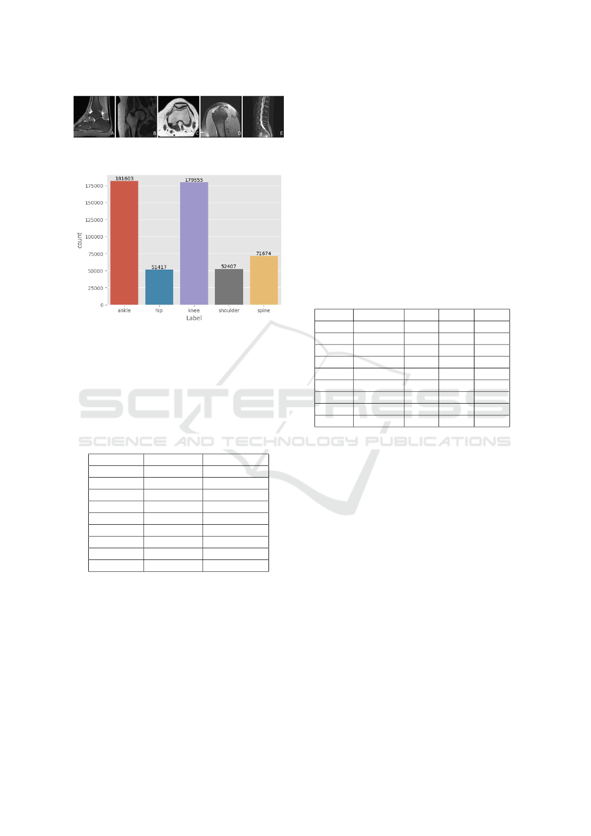
Figure 3: Images samples from dataset A- Ankle, B- Hip,

C- Knee, D- Shoulder, E- Spine.

Figure 4: Dataset classes repartition.

distribution of 65%, 25%, and 10%. Subsequently,

to form the sub-datasets, we perform a random shuf-

ﬂe within the base training dataset to extract the de-

sired quantity of data. Following this, we conduct an-

other random shufﬂe within the validation dataset to

obtain 30% of the sub-training set for the ﬁnal valida-

tion dataset.

Table 1: Number of datas in each training.

Percentage Training set Validation set

100 348 824 134 161

70 244 176 73 252

50 174 412 52 323

30 104 647 31394

10 34 882 10 464

5 17 441 5232

3 10 464 3139

1 3 488 1046

0.5 1 744 523

3.2 Training Parameters

For training, data augmentation is not employed. The

input image size for the network is set to 224x224,

with a ﬁxed batch size of 32. The learning rate is

established at 1e-4, and models are trained for 30

epochs. The optimizer used is Adam, and Cross

Entropy serves as the loss function. The metrics

monitored during training include loss, accuracy, and

AUC.

Training involves shufﬂing the dataset, while vali-

dation does not shufﬂe. The best model is saved when

the validation loss decreases. During inference on the

test dataset, the best model is used.

3.3 Setup

We aim to design a minimalist CNN for high-

performance training with mainstream computational

resources. All training is conducted on a laptop

equipped with an Intel Core i9 12th generation pro-

cessor, 32 GB of RAM, and an NVidia GeForce

RTX3070ti GPU with 8 GB of video memory.

4 RESULTS

Table 2: Training time per epoch for each model and each

subdataset in hour and minutes.

%Data miniCNN UEnc RN18 RN50

0.5 00:04 00:12 00:05 00:08

1 00:06 00:23 00:07 00:14

3 00:12 01:05 00:16 00:41

5 00:20 01:52 00:25 01:10

10 00:39 03:32 00:49 02:35

30 01:57 10:10 02:25 06:32

50 03:27 19:13 04:01 11:34

70 05:22 26:23 05:23 14:41

100 08:23 38:05 10:45 27:47

Training Time & Performances. There is a signif-

icant increase in training time depending on the net-

work and the amount of data used, as illustrated in

Figure 2. With the same amount of data, UEnc takes

more time to train than other architectures. Overall,

all models exhibit nearly similar performances for a

speciﬁc amount of data, as shown in Table 3.

However, when comparing training times to the

number of parameters in each model, RN50 outper-

forms UEnc with more parameters. Surprisingly,

miniCNN, despite its simpler architecture, demon-

strates comparable performance to RN50.

Performances & Training Stability. If the per-

formances of miniCNN are comparable to those of

RN50, it is essential to verify that models are not over-

ﬁtting or underﬁtting. For the same amount of data,

both miniCNN and RN18 exhibit less stable learning

than the U-Net encoder or RN50. Regardless of the

data quantity, RN18 displays the least stable learning

and struggles to converge easily, Figure 7.

Examining the training stability of miniCNN con-

cerning the data quantity reveals that the learning pro-

cess becomes more stable with at least 10% of the

VISAPP 2024 - 19th International Conference on Computer Vision Theory and Applications

758

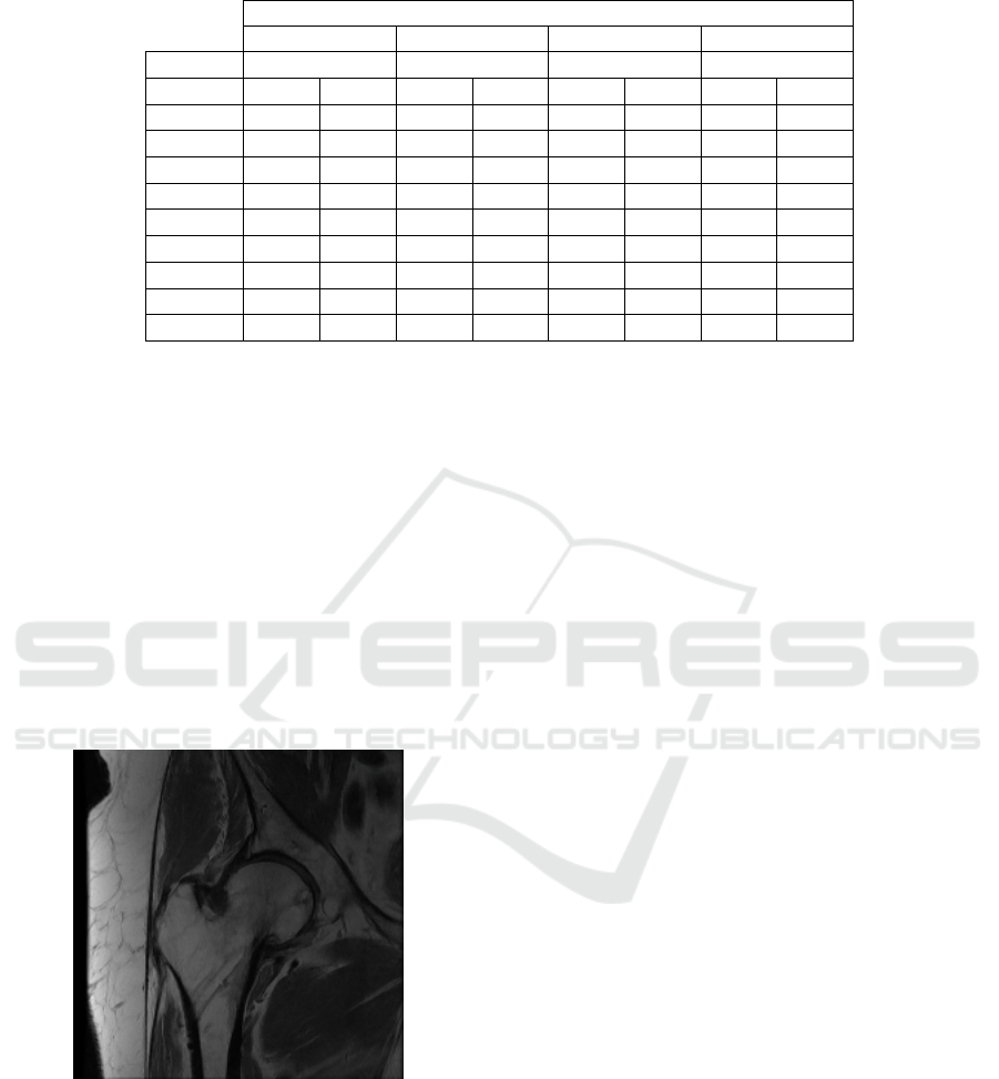
Table 3: Results of 4 models trained with different amount of datas evaluated with classical metrics (precision, AUC).

Models

miniCNN UEnc RN18 RN50

# param 948 293 18 848 325 11 179 077 23 518 277

Dataset AUC ACC AUC ACC AUC ACC AUC ACC

0.5 95.48 79.23 98.20 90.23 99.46 94.42 99.22 92.63

1 97.15 84.25 99.55 95.46 99.82 97.03 99.76 96.61

3 99.28 93.09 99.92 98.40 99.92 97.69 99.89 97.48

5 99.62 95.63 99.95 98.82 99.97 99.03 99.93 99.28

10 99.89 97.49 99.98 99.48 99.98 99.43 99.98 99.38

30 99.98 99.13 99.99 99.64 99.99 99.74 99.99 99.73

50 99.98 99.31 99.99 99.58 99.99 99.85 99.99 99.84

70 99.99 99.40 99.99 99.84 99.99 99.87 99.99 99.88

100 99.99 99.68 99.98 99.47 99.99 99.92 99.99 99.89

dataset. The same observation can be done for the

UEnc and RN50.

Performances & Grad-CAMs. The Grad-CAMs 6

associated with the last conv-block of each network

for different data quantities are presented. We aim to

determine if the learned features remain relevant with

a smaller network and fewer data. We use an image

from the test dataset to present a visual analysis of

activation maps, Figure 5. A general observation in-

dicates that the Grad-CAM activations of Uenc with a

data quantity greater than 30% of the dataset are more

precise. In contrast, the Grad-CAMs of miniCNN are

much less accurate, regardless of the data quantity.

Figure 5: Hip MRI from test dataset from RadImageNet.

5 DISCUSSION

Conv-Block Choice. For simplicity in our model

selection, we focused on U-Net and ResNet architec-

tures. However, we could explore other well-known

models like DenseNet, AlexNet, VGG in future inves-

tigations in order to provide additional comparisons.

Dataset & Classiﬁcation Tasks. We chose a spe-

ciﬁc classiﬁcation task, but it would be interesting to

test on a more complex task, such as lesion classiﬁca-

tion. This would allow us to compare our results with

RadImageNet or with other related works in medical

imaging, providing a more comprehensive and com-

plete evaluation.

Training Parameters. In this study, all parameters

were ﬁxed to evaluate the performance of different

models consistently. However, with a limited dataset,

training may be unstable. The batch size initially set

at 32 could be reduced to aid the network in better

convergence. In cases where the dataset cannot be ex-

panded due to a lack of data, data augmentation meth-

ods could enhance learning stability. Furthermore,

training was conducted for 30 epochs, but increasing

the number of epochs and incorporating early stop-

ping methods would be beneﬁcial.

Minimalist CNN as the Best Compromise. Our

minimalist CNN is not a speciﬁc network. In fact, it

represents a model from a sufﬁcient compromise be-

tween the dataset, training time, model performance,

learning quality, and the features learned by the net-

work. For instance, in our sub-dataset containing

0.5% of the dataset, the performance of miniCNN and

UEnc is lower than RN18 and RN50. The training

curves show smoother learning curves for miniCNN

than RN18 and RN50. The Grad-CAMs of miniCNN,

UEnc, and RN50 are not as relevant as those of RN18

in this context, making RN18 the minimalist CNN.

Moving on to our sub-dataset with 30% of the data, all

four architectures exhibit excellent and similar perfor-

mances, and training appears stable. In comparison to

our reference image, we observe that the Grad-CAMs

are more relevant with UEnc than with the other mod-

els. However, concerning training time, UEnc is the

Minimalist CNN for Medical Imaging Classiﬁcation with Small Dataset: Does Size Really Matter and How?

759

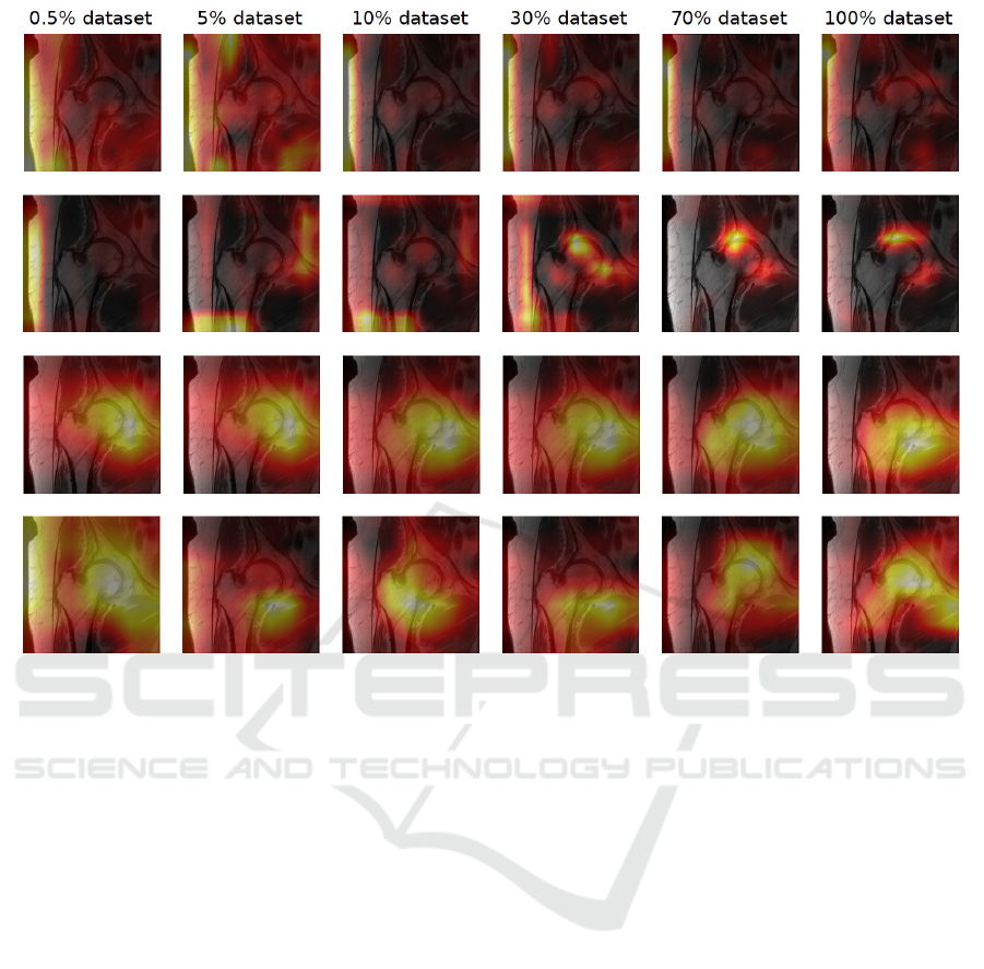
Figure 6: Grad-CAM on the last epoch for each model. Row1 - miniCNN, Row2 - UEnc, Row3- RN18, Row4 - RN50.

slowest model to train. Therefore, to determine our

minimalist CNN, a compromise must be done be-

tween training time and the quality of explanations

provided by Grad-CAMs.

Grad-CAMs. Provide a ﬁrst comprehension ele-

ment about how the network predicts a class. In ad-

dition to visual analysis, a quantitative evaluation of

Grad-CAMs could be conducted to ensure the rele-

vance of the produced Grad-CAMs. There are various

evaluation methods, some involving model retraining

and others not. For example, an image perturbation

method known as ROAD (Remove and Debias) (Rong

et al., 2022), combines Most Relevant First (MORF)

and Least Relevant First (LERF) methods. MORF re-

moves the highest attention pixels ﬁrst, while LERF

removes the least attention pixels ﬁrst.

6 CONCLUSIONS

In this preliminary study, we have demonstrated our

ability to design a minimalist CNN adapted to a spe-

ciﬁc medical image classiﬁcation task and dataset.

The results indicate that our minimalist CNN achieves

comparable performance to larger CNN architectures

with mainstream computational resources. This high-

lights the potential of our approach in establishing a

pipeline to design a minimalist CNN. Moving for-

ward, we aim to further reﬁne our minimalist CNN

by incorporating more comparison criteria in the pro-

cess such as explainability method. This could help

ensure not only performance but also a deeper un-

derstanding of the learned features. More precisely,

we could use the quality evaluation of the features

learned by the network and integrate this evaluation

as an additional metric to improve the architecture of

our network, keeping it as small as possible.

In future works, we will apply our Minimalist

CNN design to other medical image datasets and dif-

ferent classiﬁcation tasks such as speciﬁc or general

abnormalities classiﬁcation. To address the challenge

of limited data availability we will evaluate the in-

ﬂuence of data augmentation and transfer learning

on our model. Furthermore, we need to test more

CNN architecture to design our minimalist CNN.

Even though a lot of current studies are based on

big complex architectures trained to answer multiple

tasks, it’s interesting to design smaller models. We

will compare our minimalist CNN with bigger models

on the same tasks and dig deeper into our evaluation

process to ensure interpretability and robustness.

VISAPP 2024 - 19th International Conference on Computer Vision Theory and Applications

760

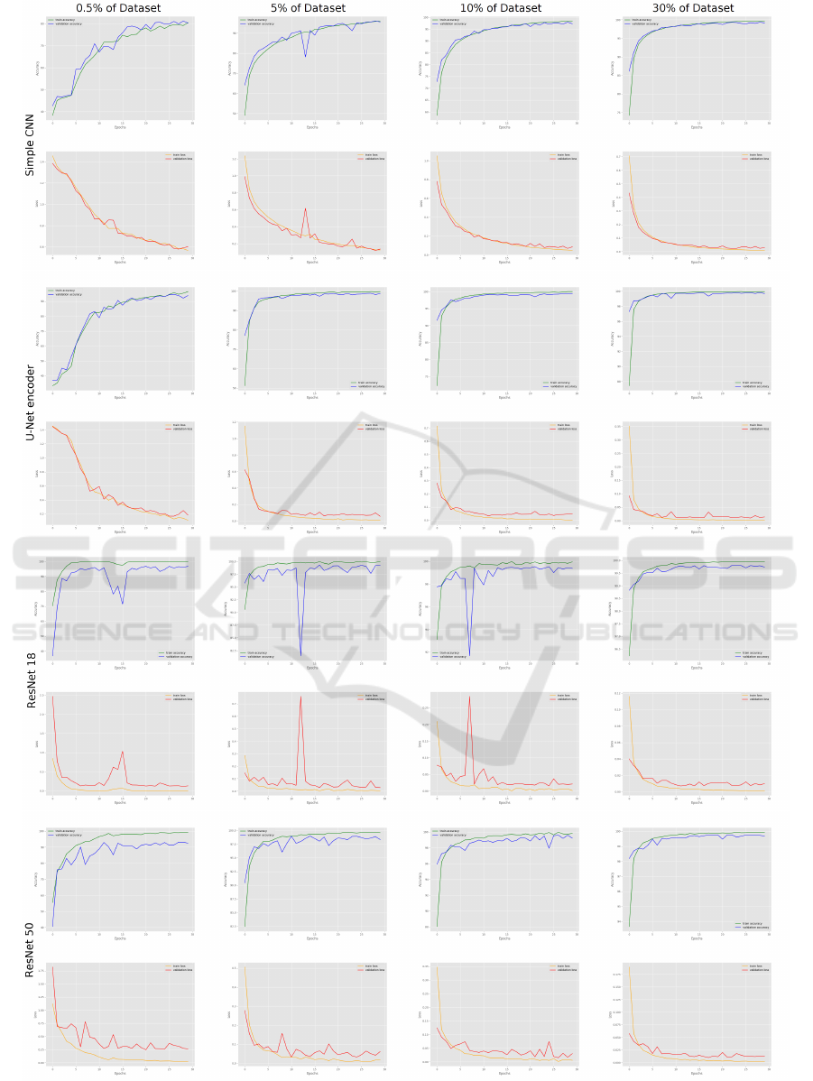
Figure 7: Training curves.

Minimalist CNN for Medical Imaging Classiﬁcation with Small Dataset: Does Size Really Matter and How?

761

ACKNOWLEDGEMENTS

This research was supported by GE Healthcare. We

thank Nicolas Gogin for comments that greatly im-

proved this paper.

We would also like to show our gratitude to the

reviewers for their comments and advices.

REFERENCES

Albelwi, S. and Mahmood, A. (2017). A framework for de-

signing the architectures of deep convolutional neural

networks. Entropy.

Bien, N., Rajpurkar, P., Ball, R. L., Irvin, J., Park, A., Jones,

E., Bereket, M., Patel, B. N., Yeom, K. W., Shpan-

skaya, K., et al. (2018). Deep-learning-assisted di-

agnosis for knee magnetic resonance imaging: devel-

opment and retrospective validation of mrnet. PLoS

medicine.

Cao, X. (2015). A practical theory for designing very deep

convolutional neural networks. Unpublished Techni-

cal Report.

Fei-Fei, L., Deng, J., and Li, K. (2009). Imagenet: Con-

structing a large-scale image database. Journal of vi-

sion.

Gao, L., Zhang, L., Liu, C., and Wu, S. (2020). Handling

imbalanced medical image data: A deep-learning-

based one-class classiﬁcation approach. Artiﬁcial in-

telligence in medicine.

He, K., Zhang, X., Ren, S., and Sun, J. (2016). Deep resid-

ual learning for image recognition. In Proceedings of

the IEEE conference on computer vision and pattern

recognition, pages 770–778.

Kim, H. E., Cosa-Linan, A., Santhanam, N., Jannesari, M.,

Maros, M. E., and Ganslandt, T. (2022). Transfer

learning for medical image classiﬁcation: a literature

review. BMC medical imaging.

Krizhevsky, A., Hinton, G., et al. (2009). Learning multiple

layers of features from tiny images.

Krizhevsky, A., Sutskever, I., and Hinton, G. E. (2012). Im-

agenet classiﬁcation with deep convolutional neural

networks. Advances in neural information processing

systems, 25.

LeCun, Y., Bottou, L., Bengio, Y., and Haffner, P. (1998).

Gradient-based learning applied to document recogni-

tion. Proceedings of the IEEE, 86(11):2278–2324.

LeCun, Y., Cortes, C., and Burges, C. (2010). Mnist hand-

written digit database. ATT Labs [Online]. Available:

http://yann.lecun.com/exdb/mnist.

Mei, X., Liu, Z., Robson, P. M., Marinelli, B., Huang, M.,

Doshi, A., Jacobi, A., Cao, C., Link, K. E., Yang, T.,

et al. (2022). Radimagenet: an open radiologic deep

learning research dataset for effective transfer learn-

ing. Radiology: Artiﬁcial Intelligence.

Ramaswamy, H. G. et al. (2020). Ablation-cam: Vi-

sual explanations for deep convolutional network via

gradient-free localization. In proceedings of the

IEEE/CVF winter conference on applications of com-

puter vision.

Rizk, B., Brat, H., Zille, P., Guillin, R., Pouchy, C., Adam,

C., Ardon, R., and d’Assignies, G. (2021). Menis-

cal lesion detection and characterization in adult knee

mri: a deep learning model approach with external

validation. Physica Medica.

Rong, Y., Leemann, T., Borisov, V., Kasneci, G., and Kas-

neci, E. (2022). A consistent and efﬁcient evalua-

tion strategy for attribution methods. arXiv preprint

arXiv:2202.00449.

Ronneberger, O., Fischer, P., and Brox, T. (2015). U-

net: Convolutional networks for biomedical image

segmentation. In Medical Image Computing and

Computer-Assisted Intervention–MICCAI 2015: 18th

International Conference, Munich, Germany, October

5-9, 2015, Proceedings, Part III 18. Springer.

Selvaraju, R. R., Cogswell, M., Das, A., Vedantam, R.,

Parikh, D., and Batra, D. (2017). Grad-cam: Visual

explanations from deep networks via gradient-based

localization. In Proceedings of the IEEE international

conference on computer vision.

Simonyan, K. and Zisserman, A. (2014). Very deep con-

volutional networks for large-scale image recognition.

arXiv preprint arXiv:1409.1556.

Wasay, A. and Idreos, S. (2020). More or less: When and

how to build convolutional neural network ensembles.

In International Conference on Learning Representa-

tions.

Zavalsız, M. T., Alhajj, S., Sailunaz, K.,

Ozyer, T., and Al-

hajj, R. (2023). A comparative study of different pre-

trained deeplearning models and custom cnn for pan-

creatic tumor detection. International Arab Journal of

Information Technology.

VISAPP 2024 - 19th International Conference on Computer Vision Theory and Applications

762