Machine Learning for Predicting Traffic and Determining Road Capacity
Alex Lewis
1
, Rina Azoulay
2
and Esther David
3
1
Department of Data Mining, Jerusalem College of Technology, Jerusalem, Israel
2
Department of Computer Science, Jerusalem College of Technology, Jerusalem, Israel
3
Department of Computers, Achva Academic College, Beer Tuvia, Israel
Keywords:
Traffic Forecasting, Capacity Estimation, Machine Learning.
Abstract:
This study proposes the use of machine learning techniques to predict traffic speed based on traffic flow and
other road-related features, utilizing the California Freeway PeMS traffic dataset. Extensive research has been
dedicated to the prediction of road speed; however, the primary challenge lies in accurately forecasting speed
as a function of traffic flow. The learning methods compared include linear regression, K-nearest neighbors
(KNN), decision trees, neural networks, and ensemble methods. The primary objective of this research is to
develop a model capable of estimating road capacity, a crucial factor in designing an auction system for road
usage. The findings reveal that the performance of each algorithm varies with the selection of features and the
volume of data available. The results demonstrate that ensemble methods and KNN surpass other models in
accuracy and consistency for predicting traffic speed. These models are then employed to create a flow-speed
graph, which aids in determining road capacity.
1 INTRODUCTION
Transportation plays a vital role in modern society,
facilitating travel, the movement of goods, and the
connection of people and places. Intelligent Trans-
port Systems (ITS) aim to enhance transportation by
bringing together various elements such as vehicles,
drivers, passengers, road operators, and managers in a
way that interacts with the environment. The primary
goals of ITS are to decrease the number of road fatal-
ities and injuries, improve the efficiency of vehicles
and traffic networks, and reduce pollution(Williams,
2008).
An important aspect of traffic assignment is esti-
mating road capacity, defined as the maximum num-
ber of vehicles passing through a specific point within
a time period, considering existing road, traffic, and
control conditions (Reilly, 1997).
Traditionally, transportation capacity assessment
has relied on static statistical models from a civil engi-
neering perspective, which depend on factors such as
the number of lanes, road width, the free flow speed,
etc. Conversely, machine learning and deep learn-
ing models can assess road capacity based on real-
time data, providing traffic management systems with
a more precise understanding of network conditions,
enhancing traffic control, and reducing overall travel
time.
This study aims to construct machine learning
and deep learning models that estimate road capacity
based on current speed predictions. Our regression
models account for factors that impact speed, such as
traffic flow and other relevant features. Rather than
projecting specific capacity thresholds, we seek to ex-
plore the interplay between flow, speed, and other
variables, empowering road planners to determine op-
timal capacity for their desired speed. In the future
these models will be combined with different opti-
mization tools such as reinforcement learning and dif-
ferent search methods in order to control the traffic
optimally.
The motivation for our research is to develop a
comprehensive road network model that can capture
the dynamics and capacity of individual roads. This
model will serve as a foundation for future research,
specifically focusing on the creation of an auction sys-
tem for road entry. By leveraging the speed prediction
models developed in this study and integrating them
with the aforementioned optimization tools, the auc-
tion system will effectively assess the capacity of each
road and facilitate the allocation of slots through var-
ious auction mechanisms. This integrated approach
will contribute to improved road management and re-
source allocation in transportation systems.
1162
Lewis, A., Azoulay, R. and David, E.
Machine Learning for Predicting Traffic and Determining Road Capacity.
DOI: 10.5220/0012451900003636
Paper published under CC license (CC BY-NC-ND 4.0)
In Proceedings of the 16th International Conference on Agents and Artificial Intelligence (ICAART 2024) - Volume 3, pages 1162-1169
ISBN: 978-989-758-680-4; ISSN: 2184-433X
Proceedings Copyright © 2024 by SCITEPRESS – Science and Technology Publications, Lda.

The paper begins with a literature review dis-
cussing the use of machine learning in traffic pre-
diction and traditional capacity estimation methods.
The methods chapter explains various approaches for
speed prediction, followed by a results chapter dis-
cussing the obtained outcomes. Utilizing the mod-
els described, a capacity estimation model is devel-
oped and explained in the subsequent chapter. The
paper concludes by highlighting potential future re-
search directions in the field.
2 LITERATURE REVIEW
Road capacity refers to the number of vehicles that
can pass a given point during a specific period un-
der prevailing roadway, traffic and control conditions
(Reilly, 1997) There are many factors that affect road
capacity such as external conditions including the
weather, visibility and road lighting. (Chung et al.,
2006) Furthermore, road density (number of cars on
the road) affects the capacity. Namely, if a road is
congested, the number of cars that can enter the road
without creating further congestion is much lower
than the general capacity. (Chen, 2002)
The HCM (Highway Capacity Manual) (Reilly,
1997), a TRB (Transportation Research Board) pub-
lication in the US, provides guidelines and compu-
tational procedures for assessing highway facilities’
capacity and quality of service. The free flow speed
(FFS) is the theoretical speed of traffic when no ve-
hicles are present, and can be calculated using HCM
formulas that account for features such as lane width
and ramp density (Reilly, 1997). The FFS is influ-
enced by both intrinsic and environmental factors,
such as road width and weather conditions (Kyte
et al., 2000). Since the HCM propose a constant
equation for calculating road capacity based on free
flow speed, it fails to incorporate external and spatio-
temporal factors.
In our research we used the California Freeway
Performance Management System, a system that col-
lects real-time data from all the highways in Califor-
nia. The data is collected by over 40,000 sensors
spanning over 20,000 road segments. This database
includes data such as the average speed, flow rate and
occupancy for every 30 seconds on all the highways,
and has calculated values such as the average delay on
each of the roads (Chen, 2002). Many of the recent
works conducted on traffic prediction have been done
with data obtained from the PeMS (Tedjopurnomo
et al., 2020).
Traditional time series techniques have been used
for traffic speed and flow prediction. This include the
ARIMA (Billings and Yang, 2006) (Lee and Fambro,
1999) and it’s variants (SARIMA, ARIMAX, etc.)
(Ghosh et al., 2007) and Kalman filtering(Kumar,
2017). Moreover, Machine Learning and Deep Learn-
ing have been used in many different transportation
problems studies(Haghighat et al., 2020). Regression
techniques such as linear regression and logistic re-
gression were used for traffic flow prediction(Lonare
and Ravi, 2020). Multi-variate regression has also
been used for congestion prediction (Liu et al., 2020).
Other models such as SVM have been used for traffic
volume prediction (Mingheng et al., 2013) and deci-
sion trees have also been used for congestion predic-
tion (Tamir et al., 2020).
With the recent developments in deep learning,
there has been a lot of traffic flow and traffic speed
prediction done using deep learning (Tamir et al.,
2020). On top of the regular data used as input of
a neural network, there are specific models that uti-
lize the spatial and temporal dimensions of the data.
Spatial models use deep learning frameworks such
as CNN(Song et al., 2017) that use the geographi-
cal data in order to build the model. Temporal mod-
els employ deep learning frameworks such as RNN
and LSTM(Tian et al., 2018) that make use of his-
toric data in order to improve the prediction. There
are hybrid models that combine both spatial and tem-
poral data such as the CNN-LSTM hybrid model(Cao
et al., 2020).
Graph Neural Networks (GNNs) are deep learn-
ing methods designed to perform inference on data
described by graphs. GNNs are neural networks that
can be directly applied to graphs, and provide an easy
way to implement node-level, edge-level, and graph-
level prediction tasks. GNNs do not only have the
ability to learn using each of the segments features,
but can also catch the connections between the differ-
ent road segments using spatial data.
Extensive research has focused on predicting road
speed, however the difference between most research
and our research is that we are attempting to accu-
rately forecast speed as a function of traffic flow, and
utilizing this model for simulated data that we create
for the capacity model.
The definition of road capacity is the maximum
number of vehicles or amount of traffic flow that a
roadway can accommodate effectively and efficiently
within a given time period. In the review of the re-
search conducted in this field, we found only one
study (Huo et al., 2022) on capacity estimation using
deep learning. The error function for the network was
calculated by using the travel time as a function of
the road capacity and the error value is the difference
between the predicted travel time and the real travel
Machine Learning for Predicting Traffic and Determining Road Capacity
1163

time. The present study is different from the work
conducted by Huo et al. (Huo et al., 2022) in that a
precise quantification of the road capacity is not pro-
vided. Instead, we seek to understand the traffic flow
in relation to velocity and leverages the advantages
of spatio-temporal data, rendering it more dynamic in
nature, which will allow more flexibility for the auc-
tion system.
3 MACHINE LEARNING
METHODS FOR SPEED
PREDICTION
The goal of the model is to accurately predict the
speed of the leftmost lane for each road segment as a
function of the different input features chosen. To ac-
complish this, we employed various machine learning
algorithms, namely decision trees, random forest, k-
Nearest Neighbors (k-NN) regressor, neural networks
, and linear regression. By applying these algorithms,
we aimed to capture the underlying patterns and rela-
tionships within the data and leverage them for accu-
rate speed prediction.
Our research employs two distinct methodologies
for the analysis. The first methodology involves con-
structing machine learning models that utilize data
from all segments collectively. In contrast, the second
methodology focuses on developing individual ma-
chine learning models for each segment. By exploring
these two approaches, we aim to investigate the com-
parative effectiveness and performance of both cen-
tralized and decentralized modeling strategies in cap-
turing the complexities of the data.
In the first methodology, we gathered traffic data
from multiple segments and used data from all the
segments to help with the prediction (the segment id
was not part of the input for the model). This holistic
approach allowed us to capture the collective traffic
dynamics and identify broader trends across the road
network. Utilizing the aforementioned algorithms, we
trained models on this dataset to predict the speed on
the roads.
In the second methodology, we focused on the in-
dividual segment level, where we isolated the data
from each segment to predict the speed specific to
that segment. This approach provided insights into
the localized factors influencing road speed, allowing
for more targeted predictions. Similar to the previous
methodology, we employed the decision trees, ran-
dom forest, k-NN regressor, SVR, and linear regres-
sion algorithms to build segment-specific models.
To capture the temporal aspect, we introduced
lag features that integrate time-series information.
Specifically, these lag features were constructed by
considering the flow and speed values from the pre-
vious three time slots, encompassing both the entire
road segment and specifically the first lane. Further-
more, we incorporated the hour of travel as an ad-
ditional feature, which was represented as an integer
between 0 and 23.
In order to investigate the influence of different in-
put features on our predictive model, we conducted a
series of experiments utilizing various combinations
of inputs. Our objective was to systematically vary
the input variables and evaluate whether specific at-
tributes resulted in improved outcomes, meaning bet-
ter MSE and R2 and also models that generalize well
to unseen data. We employed three distinct sets of
input variables for this purpose.
The first set focused on road-specific information,
encompassing factors such as the number of lanes,
road type obtained from the Pems database, and flow
data. The flow data consisted of the current flow, as
well as lag features representing flow from the previ-
ous three time slots.
For the second set, we expanded the feature space
by including the lag features for road speed from the
previous three time slots. This addition allowed us to
capture temporal dependencies in the speed data.
In the third set, we introduced the free flow speed
to the first input set. This augmentation enhanced the
speed-related information without the need to incor-
porate the most recent history of speed. There was no
reason to use this input set for the second methodol-
ogy since the free flow speed would be equal for all
of the data because the learning is on each segment
individually.
We had a specific motivation for conducting an ex-
periment using an input set solely comprised of flow
lag features, excluding the speed features. The ra-
tionale behind this decision was to evaluate whether
our model could achieve satisfactory performance by
solely relying on flow values. By doing so, we aimed
to develop a capacity model that could accurately pre-
dict optimal capacity without relying on knowledge
of recent speed variations on the road. This approach
would allow us to create a model based on the flow
data and other constant features, providing us with the
capability to estimate optimal capacity independently
of recent speed information. Utilizing speed methods
can be useful for a live system with real data, and the
values for the MSE and R2 can also set a benchmark
for the accuracy that can be acheived.
ICAART 2024 - 16th International Conference on Agents and Artificial Intelligence
1164

3.1 Learning Methods
Linear Regression. A statistical method for modeling
the relationship between a dependent variable and one
or more independent variables. It assumes a linear
relationship between the variables and aims to find the
best-fit line that represents the data.
K-nearest Neighbors (KNN). A non-parametric
machine learning algorithm used for classification or
regression. It works by finding the K nearest data
points to a given query point and using their la-
bels/values to make a prediction.
Neural Network. A type of machine learning al-
gorithm modeled after the structure and function of
the human brain. It consists of layers of intercon-
nected nodes (neurons) that process information and
learn from data through a process called backpropa-
gation.
Decision Trees. A machine learning algorithm
that uses a tree-like structure to model decisions and
their possible consequences. Each node in the tree
represents a decision based on a feature, and each
branch represents the possible outcomes based on the
decision.
Random Forest. A type of ensemble machine
learning algorithm that combines multiple decision
trees to improve prediction accuracy and reduce over-
fitting. It works by building multiple decision trees
on random subsets of the data and aggregating their
predictions.
3.2 The Data
The research was carried out using data from the
California Freeway PeMS (Performance Management
System), a system that collects real-time data from
all the highways in California. Over 40,000 sensors
spanning over 20,000 road segments collect the data
which include the average speed, the flow rate and the
occupancy for every 30 seconds on each of the road
segments, as well as calculated values such as aver-
age delays (Chen, 2002). The data used in our basic
model was obtained from District 3 in California and
spanned the whole of the month of September 2022,
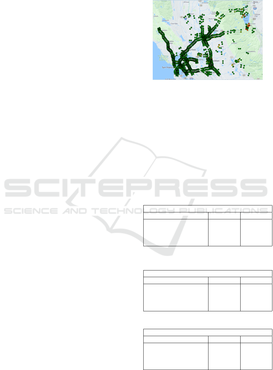
and the segments in the district can be seen in Figure
1. Our dataset comprises 12 million observations, and
we used a 75:25 train-test split after eliminating some
of the data as part of the pre-processing stage.
4 RESULTS
In this section, we want to discuss the results of the
different models built and how we can use them for
Figure 1: PeMS District 3 segments.
capacity models. We measured the results of the mod-
els using the value of the mean squared error (MSE)
and the R2 score.
The first three tables are the tables that utilized the
first methodology, where the models learn from all the
segment’s data together. The results for the first input
set, the input set that includes the speed lag features
can be seen in table 1, the results for the second input
set - the input set with flow features and without any
speed related features can be seen in table 2 and the
results for the third set, the set that includes the ffs as
the speed related feature can be seen in table 3.
Table 1: First methodology, first input set (speed lag fea-
tures).
Regression Scores - first input set
Model MSE R2
Decision Tree 3.59 0.937
Random Forest 2.98 0.948
Nearest Neighbors 3.43 0.940
Neural Network 3.20 0.944
Table 2: First methodology, second input set (no speed re-
lated features).
Regression Scores - second input set
Model MSE R2
Decision Trees 39.38 0.315
Random Forest 36.71 0.362
Nearest Neighbors 35.19 0.352
Neural Network 42.64 0.275
Table 3: First methodology, third input set.
Regression Scores - third input set (ffs feature)
Model MSE R2
Decision Tree 24.98 0.56
Random Forest 19.94 0.65
Nearest Neighbors 20.47 0.64
Neural Network 27.54 0.52
Machine Learning for Predicting Traffic and Determining Road Capacity
1165

The results for the second methodology for speed
prediction, predicting the speed using only data from
each individual segment, are presented in the follow-
ing tables. Table 4 shows the results for the first input
set, the input set with speed related features and table
5 shows the results for the second input set, the input
set without any speed related features.
Table 4: Second methodology, first input set.
Regression Scores -speed lag features
Model Mean
MSE
Median
MSE
Mean
R2
Median
R2
Linear Regres-
sion
3.71 2.31 0.71 0.80
Decision Trees 4.17 2.50 0.61 0.79
Random Forest 3.35 2.00 0.70 0.83
Nearest Neigh-
bors
3.66 2.23 0.75 0.83
Neural Net-
work
4.92 3.04 0.6 0.78
Table 5: Second methodology, second input set.
Regression Scores - no speed related features
Model Mean
MSE
Median
MSE
Mean
R2
Median
R2
Linear Regres-
sion
21.81 10.4 0.28 0.26
Decision Trees 16.23 7.98 0.34 0.38
Random Forest 13.19 6.52 0.46 0.48
Nearest Neigh-
bors
13.29 6.76 0.45 0.47
Neural Net-
work
4.92 3.04 0.6 0.78
The findings obtained indicate that in the context
of individual segment-based predictions, basic ma-
chine learning techniques like linear regression ex-
hibit comparable performance to more sophisticated
algorithms such as random forest and neural network.
This observation suggests that the data pertaining to
each individual segment is not characterized by sub-
stantial complexity.
We experimented with different values for the
amount of neighbors from which to learn in the KNN
algorithm, here too there wasn’t much difference be-
tween the results for different parameters. We ex-
perimented with different values for the depth of the
tree, where the optimal value changed for each of the
different feature input sets. Additionally, we experi-
mented both with the maximum depth and number of
estimators for the random forest algorithm. The MSE
value for the different depths were pretty similar and
varied for each of the different input sets.
Upon analyzing the outcomes of the second in-
put set, the input set with no speed related features,
it becomes evident that relying solely on the flow lag
features does not suffice to generate a robust model.
This limitation could be attributed to the insufficient
availability of comprehensive data pertaining to each
road’s characteristics, necessitating the inclusion of
speed lag features. The models may lack adequate
temporal context when considering only the three
most recent flow values. Incorporating additional
time series features and utilizing specialized tempo-
ral models such as CNN and RNN could potentially
enhance the model’s performance by capturing more
intricate temporal patterns.
Notably, the results obtained from the third input
set demonstrate a substantial improvement in perfor-
mance upon incorporating speed data, even though it
does not encompass the most recent historical speed
information. This finding underscores the signifi-
cance of incorporating speed-related information, as
it yields significant enhancements in model accuracy,
despite not relying on the immediate speed history.
The first methodology that learns from all the seg-
ments collectively proves to perform as well as the
second which just learns from each segment sepa-
rately, this shows us that models can generalize pretty
well over a road network given enough data and fea-
tures, and the models generalize well for the whole of
the road network.
5 THE CHALLENGE OF
CAPACITY PREDICTION
According to the Highway Capacity Manual (HCM),
the definition of road capacity is the maximum num-
ber of vehicles or amount of traffic flow that a
roadway can accommodate effectively and efficiently
within a given time period, taking into account fac-
tors such as lane width, number of lanes, geometric
design, signal timings, and other operational charac-
teristics (Reilly, 1997).
The capacity is calculated using the following for-
mula:
Capacity = MSFE * PHF * N * fhv * fp (Reilly,
1997)
Where: PHF = peak-hour factor which represents
the variation in traffic flow within an hour fHV = an
adjustment factor for the presence of “heavy” vehi-
cles fp = an adjustment factor to account for the fact
that all drivers of the facility may not be commuters
or regular users N = number of lanes in the given di-
rection of flow MSFe = maximum possible flow rate
we can have to still be at level of service e
The first four variables are variables that can’t be
changed by the road planner, and the last the MSFE
is the maximum service flow rate that is required to
ICAART 2024 - 16th International Conference on Agents and Artificial Intelligence
1166

Figure 2: HCM capacity table (Reilly, 1997).
maintain a certain speed. The values for these can be
found in the HCM table in figure 2:
With these guidelines the capacity doesn’t depend
on the amount of cars in the road or the previous
speeds and flows observed on the road. Using ma-
chine learning algorithms can provide us with much
more accurate values for this and allows a system to
be dynamic and change the capacity according to the
exact current road conditions. On top of this, the ma-
chine learning algorithm allows us to find optimize
the capacity for each of the roads, and find the values
of the speed and flow that allow for maximizing the
distance traveled on the road which we defined as our
utility function, but this could be expanded to other
utility functions too.
For the sake of this research, we are going to de-
fine the road’s capacity as the flow that produces the
highest utility, where the utility function is the amount
of kilometres covered on the road, which is the mul-
tiplication of the speed and flow. To estimate road
capacity, we developed a procedure based on the top
performing machine learning models built in the pre-
vious stage and used them to predict the speed under
different conditions. We built these models based on
both input sets - the first including road metadata and
flow features and the second that includes speed fea-
tures too, we did this with both methodologies used
in the previous section - i.e using all segments data
for prediction and prediction using only the individ-
ual segment.
To determine the optimal flow for each road, we
adopted a two-stage approach. In the first stage, we
created a list of optional flows and speeds for each
road (depending on the input set), considering a max-
imum flow of the road as the maximum flow observed
in the dataset for that road. Subsequently, we utilized
the trained random forest model to predict the cor-
responding speeds for each of these flows. A mini-
mum optional speed threshold was defined, and the
flow that maximized the utility function, which is the
Figure 3: Flow to speed graph for road 313114, prediction
using random forest with 5 different input sets and HCM.
product of flow and speed i.e the total distance trav-
eled on the road, was selected as the optimal flow.
We found the corresponding speeds for the differ-
ent values for the maximum flow service rate that’s
shown in the HCM table in figure 2 using the dif-
ferent machine learning algorithms used in the pre-
vious chapters. Using the first input set - the set that
includes the previous speeds proved to overfit to the
speed features and these algorithms didn’t generalize
well to the hypothetical situations. Because of this,
we tried to improve the second input set with other
features that don’t include the previous speed values.
We added the free flow speed for each of the segments
that was calculated by taking the mean speed between
00:00 and 01:00 every day. This improved the MSE
to 25 and the R2 to 0.56, and in future work we want
to improve this even further, so that we can produce a
model that learns just from the flow and constant vari-
ables that define the road and make sure that we don’t
use the speed features.
In the following table we can see an example of
a comparison between the capacity used by apply-
ing the HCM capacity equation and the random for-
est and KNN models using the 5 different models - 2
input sets for the individual based models and 3 for
the generalized based models explained in the previ-
ous section. We have assumed the PHF is 0.92 (Tarko
and Perez-Cartagena, 2005) and that no modifications
need to be made for heavy vehicles and that all drivers
are regular commuters. This has been done on a road
with a FFS of 74mph and we used the HCM guide-
lines for 120 kmh which is almost exactly equivalent.
The road we picked is road with the ID 313114. The
results for the random forest models are presented in
figure3 and the results for the KNN models are pre-
sented in figure 4.
Based on the observed outcomes, it is evident that
the utilization of speed features in the models leads to
overfitting to the particular road data, thereby hinder-
ing their ability to generalize effectively. Moreover,
the graph depicts a consistent trend where all models
fail to adequately capture traffic dynamics, particu-
larly where the value of the flow is high. This inade-
Machine Learning for Predicting Traffic and Determining Road Capacity
1167

Figure 4: Flow to speed graph for road 313114, prediction
using KNN with 5 different input sets and HCM.
quacy may arise from the limited availability of rele-
vant data, high traffic data isn’t as common as normal
traffic data. To elucidate this phenomenon, we can
invoke the well-known concept that correlation does
not necessarily imply causation. In this context, the
models that incorporate speed features excel in cap-
turing correlation patterns but fall short in capturing
the underlying causal relationships.
We can further discern that the K-nearest neigh-
bors (KNN) model outperforms the random forest
model in the right region of the graph. This superi-
ority can be attributed to the KNN model’s ability to
learn from very similar examples, allowing it to ef-
fectively learn from rarer data instances, in contrast
to the random forest model, which learns from the
entirety of the data. In light of this, it becomes ev-
ident that the KNN model’s performance advantage
stems from its specific learning characteristics and its
ability to leverage similar and rare data patterns. The
advantage of the KNN is that it succeeds in learning
well even when the value of the flow is high and it the
model doesn’t underfit. However, the compute time
for the test set is very high and also we can observe
that for the first methodology the model doesn’t learn
the base speed well enough.
6 CONCLUSIONS
In this study, we aimed to estimate road capacity us-
ing machine learning and deep learning models based
on real-time data and speed predictions. Our regres-
sion models accounted for factors such as traffic flow
and other relevant features that impact speed. Rather
than projecting specific capacity thresholds, our mod-
els explored the interplay between flow, speed, and
other variables, empowering road planners to deter-
mine optimal capacity for their desired speed. By
leveraging these models in combination with opti-
mization tools, we aimed to improve road manage-
ment and resource allocation in transportation sys-
tems. Our research introduces specifically a speed
prediction model using the flow data.
To construct our models, we employed vari-
ous machine learning algorithms, including decision
trees, random forest, k-Nearest Neighbors (k-NN) re-
gressor, and linear regression. Through two distinct
methodologies, we investigated the effectiveness of
centralized and decentralized modeling strategies in
capturing the complexities of traffic dynamics. Tem-
poral dependencies were considered by incorporating
lag features that integrated time-series information.
We systematically varied the input variables to evalu-
ate their influence on the predictive models, focusing
on road-specific information, speed lag features, and
the addition of free flow speed. The evaluation of our
models was based on metrics such as Mean Squared
Error (MSE) and R2 score.
Based on our findings, we concluded that machine
learning and deep learning models, in conjunction
with optimization tools, hold promise in accurately
estimating road capacity. By considering the dynam-
ics of individual roads and incorporating real-time
data, our models provide insights into localized fac-
tors influencing road speed. This research contributes
to the field of transportation systems by providing a
comprehensive road network model and showcasing
the potential of using machine learning for determin-
ing road capacity.
Future research endeavors are expected to signif-
icantly augment the existing model’s predictive ca-
pabilities by integrating a more comprehensive range
of external conditions. The inclusion of supplemen-
tary data sets, such as weather and spatio-temporal
data, holds tremendous promise for further enhanc-
ing the model’s performance. Combining ensemble
methods using decision trees together with neural net-
works has showed improvements even with tabular
data (Shwartz-Ziv and Armon, 2021) so building en-
semble models could improve results even without
adding anymore data. Moreover, incorporating the
structural layout of the road network and the inter-
dependence among roads by using spatial data and
graph neural network (GNN) architecture can po-
tentially elucidate the intricate connections between
nodes in the graph.
Furthermore, to comprehend the underlying tem-
poral structure, time series features will be integrated
into the model’s architecture. To capture the intri-
cacies inherent in the data and enable the model to
make precise predictions, the proposed research en-
deavors will utilize deep learning architectures such
as convolutional neural networks (CNNs), recurrent
neural networks (RNNs), and long short-term mem-
ory (LSTM). These architectures have demonstrated
impressive capabilities in analyzing time series data,
ICAART 2024 - 16th International Conference on Agents and Artificial Intelligence
1168

thereby enabling the model to extract relevant features
and make accurate forecasts. By integrating these
cutting-edge techniques into our model, we aim to en-
hance its predictive capabilities and offer valuable in-
sights into transportation planning and management.
Conversely, instead of using neural networks for the
temporal structure, as shown in our current findings
the random forest model performs well on time series,
and this can be combined together with the GNN for
the spatial structure as demonstrated in the following
research (Ivanov and Prokhorenkova, 2021).
Future research will incorporate spatial-temporal
models, aiming to encompass the entire network. Ad-
ditionally, advanced optimization algorithms, such as
genetic algorithms and simulated annealing, will be
employed to determine the optimal capacity for the
entire network dynamically at any given time. We
plan on using advanced optimization techniques such
as genetic algorithms and simulated annealing. Af-
ter incorporating these advanced optimization algo-
rithms, our future plan involves developing a simu-
lator that accurately replicates real traffic data. This
simulator will serve as a platform to evaluate and
compare the performance of different optimization al-
gorithms.
ACKNOWLEDGEMENTS
This research was partially supported by the ministry
of Innovation, Science & Technology, Israel.
REFERENCES
Billings, D. and Yang, J.-S. (2006). Application of the arima
models to urban roadway travel time prediction - a
case study. In 2006 IEEE International Conference
on Systems, Man and Cybernetics, volume 3, pages
2529–2534.
Cao, M., Li, V. O., and Chan, V. W. (2020). A cnn-lstm
model for traffic speed prediction. In 2020 IEEE 91st
Vehicular Technology Conference (VTC2020-Spring),
pages 1–5. IEEE.
Chen, C. (2002). Freeway performance measurement sys-
tem (PeMS). University of California, Berkeley.
Chung, E., Ohtani, O., Warita, H., Kuwahara, M., and
Morita, H. (2006). Does weather affect highway ca-
pacity? 5th International Symposium on Highway Ca-
pacity and Quality of Service, pages 139–146.
Ghosh, B., Basu, B., and O’Mahony, M. (2007). Bayesian
time-series model for short-term traffic flow fore-
casting. Journal of transportation engineering,
133(3):180–189.
Haghighat, A., Ravichandra-Mouli, V., Chakraborty, P., Es-
fandiari, Y., Arabi, S., and Sharma, A. (2020). Appli-
cations of deep learning in intelligent transportation
systems.
Huo, J., Wu, X., Lyu, C., Zhang, W., and Liu, Z. (2022).
Quantify the road link performance and capacity us-
ing deep learning models. IEEE Transactions on In-
telligent Transportation Systems.
Ivanov, S. and Prokhorenkova, L. (2021). Boost then
convolve: Gradient boosting meets graph neural net-
works. In International Conference on Learning Rep-
resentations.
Kumar, S. V. (2017). Traffic flow prediction using kalman
filtering technique. Procedia Engineering, 187:582–
587.
Kyte, M., Khatib, Z., Shannon, P., and Kitchener, F. (2000).
Effect of environmental factors on free-flow speed. In
Fourth International Symposium on Highway Capac-
ity, pages 108–119.
Lee, S. and Fambro, D. B. (1999). Application of subset
autoregressive integrated moving average model for
short-term freeway traffic volume forecasting. Trans-
portation Research Record, 1678(1):179–188.
Liu, Y., Liu, C., and Zheng, Z. (2020). Traffic conges-
tion and duration prediction model based on regres-
sion analysis and survival analysis. Open Journal of
Business and Management, 8(2):943–959.
Lonare, S. and Ravi, B. (2020). Traffic Flow Prediction Us-
ing Regression and Deep Learning Approach, pages
641–648.
Mingheng, Z., Yaobao, Z., Ganglong, H., and Gang, C.
(2013). Accurate multisteps traffic flow prediction
based on svm. Mathematical Problems in Engineer-
ing, 2013.
Reilly, W. (1997). Highway capacity manual 2000. Tr
News, (193).
Shwartz-Ziv, R. and Armon, A. (2021). Tabular data: Deep
learning is not all you need. Inf. Fusion, 81:84–90.
Song, C., Lee, H., Kang, C., Lee, W., Kim, Y. B., and Cha,
S. W. (2017). Traffic speed prediction under week-
day using convolutional neural networks concepts. In
2017 IEEE Intelligent Vehicles Symposium (IV), pages
1293–1298. IEEE.
Tamir, T. S., Xiong, G., Li, Z., Tao, H., Shen, Z., Hu, B.,
and Menkir, H. M. (2020). Traffic congestion predic-
tion using decision tree, logistic regression and neural
networks. IFAC-PapersOnLine, 53(5):512–517.
Tarko, A. and Perez-Cartagena, R. (2005). Variability of
peak hour factor at intersections. Transportation Re-
search Record, 1920:125–130.
Tedjopurnomo, D. A., Bao, Z., Zheng, B., Choudhury, F.,
and Qin, A. K. (2020). A survey on modern deep
neural network for traffic prediction: Trends, methods
and challenges. IEEE Transactions on Knowledge and
Data Engineering.
Tian, Y., Zhang, K., Li, J., Lin, X., and Yang, B. (2018).
Lstm-based traffic flow prediction with missing data.
Neurocomputing, 318:297–305.
Williams, B. (2008). Intelligent transport systems stan-
dards. Artech House.
Machine Learning for Predicting Traffic and Determining Road Capacity
1169