
Surface Extraction in Coherence Scanning Interferometry by
Gauss-Markov Monte-Carlo Method and Teager-Kaiser Operator
Fabien Salzenstein
1
and Abdel-Ouahab Boudraa
2 a
1
Universit
´
e de Strasbourg, Laboratoire ICube, 23 Rue du Loess, Strasbourg, 67037 Cedex 2, France
2
Ecole Navale/Arts et Metiers Institute of Technology, IRENav, BCRM Brest, CC 600, Brest, France
Keywords:
AM-FM Model, Teager-Kaiser Energy Operator, Gauss-Markov Process, Rugosity, Surface Extraction.
Abstract:
This work deals with the problem of surface extraction using a combination of Teager-Kaiser operators and
Gauss-Markov process in the context of coherence scanning (or white light scanning i.e, WLSI) interferometry.
Our approach defines a Markov sequence along multiple surface profiles extracting their characteristics by the
means of parameters describing the fringe signals along the optical axis, while most studies of the literature
are restricted to local extraction of signals in one-dimensional mode. Thus the interest of the proposed strategy
is to classify different surfaces present in a material, in particular the information relating to their roughness,
by exploiting the statistical dependence between neighboring points where the noise is supposed to be white
Gaussian noise. The effectiveness of our unsupervised method is illustrated on both synthetic and real images.
1 INTRODUCTION
White light scanning interferometry (WLSI) tech-
nique, has shown efficiency for computing surface
depth measurements, and specifically estimating their
roughness. A high precision is required in order to
control the fabrication techniques of new materials,
microelectronic devices and MicroElectroMechanical
Systems (MEMS) (O’Mahony et al., 2003). More-
over, the strength of the WLSI technique lies in its
ability to provide fast, robust and high resolution mea-
surements, using methods based on the AM-FM sig-
nal model representing variations in light intensity
measured along the optical axis of an interference mi-
croscope. According to this model, the height of the
surface material is simultaneously contained within
the envelope and the phase of the modulated signal.
An efficient method to extract the surface position, by
detecting the envelope peak, is the so called five sam-
ple adaptive technique which uses only five adjacent
samples along the optical axis (Larkin, 1996). Other
signal processing tools such as the Fourier trans-
form (de Groot et al., 2002), the windowed Fourier
transform (WFT) (Ma et al., 2011) or the contin-
uous wavelet transform (CWT) (Sandoz, 1997; Li
et al., 2008) have also been exploited in WLSI. Based
on these transformations, phase retrieving strategies
a
https://orcid.org/0000-0002-1864-2859
have been developed for zero optical path difference
(ZOPD) compensation by extracting the local max-
ima (ridge detection) of the CWT (resp. WFT). For
example, the CWT and the WFT are used to com-
pute the phase information at a local maximum, and
have been applied to fringe pattern analysis (Niu et al.,
2009; Kemao, 2004). Due to its implementation sim-
plicity, effectiveness, and adaptation of the AM-FM
signal model, the nonlinear Teager-Kaiser energy op-
erator (TK or TKEO) is a well suited tool in this do-
main. This operator allows a fast and local demodula-
tion of signals modeled by AM-FM functions extract-
ing the instantaneous envelope and frequency. Mara-
gos and Bovik extended this energy operator to sig-
nals of higher dimensions rendering it applicable to
real-valued grayscale images as a 2D operator (Mara-
gos and Bovik, 1995). A higher order differential en-
ergy operators, for 1D signals, has been introduced
by Maragos and Potamianos (Maragos and Potami-
anos, 1995). This work has been extended by intro-
ducing a large class of operators for both 1D signals
(Salzenstein et al., 2007) followed by their multidi-
mensional version (Salzenstein et al., 2013). On the
other hand, if these different operators efficiently es-
timate the surfaces contained in an observed piece of
material, they are not well efficient for surfaces recog-
nition due to both problems: a follow-up of the sur-
faces, and their correct estimation, specifically in the
presence of close surfaces. In order to solve these
394
Salzenstein, F. and Boudraa, A.
Surface Extraction in Coherence Scanning Interferometry by Gauss-Markov Monte-Carlo Method and Teager-Kaiser Operator.
DOI: 10.5220/0012450400003654
Paper published under CC license (CC BY-NC-ND 4.0)
In Proceedings of the 13th International Conference on Pattern Recognition Applications and Methods (ICPRAM 2024), pages 394-401
ISBN: 978-989-758-684-2; ISSN: 2184-4313
Proceedings Copyright © 2024 by SCITEPRESS – Science and Technology Publications, Lda.

challenges, we combine TKEO with a Markovian ap-
proach, by drawing on the spectral tracking carried
out in the field of astronomy, where some works pro-
vide solutions to similar problems, although the sig-
nals do not contain an additional carrier term, by ex-
ploiting Bayesian approaches using MCMC (Monte
Carlo Markov Chain) algorithms (Mazet et al., 2015).
The Bayesian methodology provides a rich frame-
work for modeling inverse problems and allows us to
define a surface decomposition and pursuit approach.
To the best of our knowledge, the problem of the de-
composition of multiple surfaces related to WLSI in-
terferometric images has not been addressed in the lit-
erature using MCMC based on Gauss-Markov model
applied on different characteristics related to each sur-
face. More precisely we describe all surfaces through
their characteristic parameters such as envelope, fre-
quency, amplitude and variance, based on a Gaus-
sian envelope model added to a carrier, in order to
regularize and better discriminate them. In reference
(Hissmann and Hamprecht, 2005; Zou et al., 2016)
Bayesian approaches has been proposed as a post-
processing, to eliminate outliers or to denoise a single
surface, introducing prior knowledge on the rough-
ness of the surface, but without Markovian modeling
of the multiple fringe characteristics, that we intro-
duce in this study. In reference (Gurov and Volynsky,
2012) a Kalman filter has been used to process fringes
along the optical axis of each slice, whereas a Markov
regularization to the phase of interferometric images
has been applied in (Wu and Boyer, 2011). Let us
summarize the main contributions of our study, in the
specific field of the WLSI interferometric imaging.
• The first contribution consists in exploiting a TK
algorithm to classify the surfaces i.e, by grouping
sites belonging to an identical surface areas, using
distance neighborhood criteria;
• The second contribution consists in introducing
an unsupervised MCMC method combined with
a Gauss-Markov model applied on characteristics
related to the fringe signal, in order to better reg-
ularize the surfaces, and estimate their roughness;
• The third contribution consists in exploiting an in-
formation compression algorithm to initialize the
MCMC method, in the context of close surfaces.
This amounts to extend the surfaces characteris-
tics in an area suspected of containing adjacent
trajectories, in particular where TKEO fails.
• The fourth contribution, inspired by the work of
Mazet al. (Mazet et al., 2015), consists of ran-
domly testing, in the MCMC procedure, the be-
longing of each site to the different surfaces ac-
cording to a distance criterion including the gra-
dient matrices. This allows the nearby surfaces to
be processed more effectively.
The remainder of the paper is organized as follows:
after the presentation of the context of the interfero-
metric data in section 2 we introduce TK algorithm
in section 3 followed by the Gauss-Markov approach
adapted to the studied problem in section 4. Unsuper-
vised MCMC approach is detailed is section 5. Fi-
nally, results on both synthetic and real images are
presented section 6. Let us notice that in this study,
the surfaces are sometimes called ’trajectories’.
2 INTERFEROMETRIC SIGNAL
A series of images is acquired with a camera at regular
intervals to give a stack of xyz images. For polychro-
matic interferometry, the total intensity is the sum of
the interferences at each wavelength. From the given
interferometric fringe signals, the objective consists
in extracting the position of the analyzed surface(s). A
typical intensity signal obtained from a digital camera
as the OPD is varied in the interferometer at a given
point (x,y) on the material surface, can be approxi-
mated along the optical z-axis by a modulated sinu-
soid as follows (Larkin, 1996):
s(x,y, z) = a(x, y,z) + b(x, y)exp
"
−
z − h(x,y)
l
c
2
#
| {z }
C(x,y,z)
×cos
4π
λ
0
(z − h(x,y))+ α(x,y)
where z is a vertical scanning position along the op-
tical axis, h(x,y) represents the height of the sur-
face, a(x,y,z) is an offset intensity containing low fre-
quency components, b(x,y) is a factor proportional to
the reflected beam intensity, and α(x, y) is an addi-
tional phase offset and C(x,y,z) is the envelope. The
parameter lc represents the coherence length of the
light source and λ
0
is the average wavelength of the
light source. Generally the phase offset varies slowly
from one point (x, y) to the next, and can be neglected,
since only relative heights of the surface matter. The
main challenge consists in determining the height at
each point of the surface by exploiting the informa-
tion provided by both the envelope and the phase si-
multaneously. Most algorithms, whether based on en-
velope detection (Larkin, 1996; Sandoz, 1997), fre-
quency domain analysis (de Groot and Deck, 1993;
de Groot et al., 2002), correlation with a reference
fringe (Chim and Kino, 1990), Hilbert transformation
(Pavli
ˇ
cek and Michalek, 2012), TK algorithm (Gianto
Surface Extraction in Coherence Scanning Interferometry by Gauss-Markov Monte-Carlo Method and Teager-Kaiser Operator
395

et al., 2016), extraction of the phase information (Guo
et al., 2011) or Kalman approach (Gurov et al., 2004),
proceed along the optical axis, for each lateral posi-
tion (x,y). Some 2D techniques have been proposed
(Gurov and Volynsky, 2012; Zhu and Wang, 2012).
In our study, we perform 2D processing data, based
on a 1D initialization. The Figure 1 represents an in-
terferometric signal in biological imaging, along the
optical axis. The numbered vertices indicate super-
imposed surfaces of materials.
Figure 1: Mineral component of the phosphate family.
3 TK ENERGY OPERATORS
TKEOs based demodulation algorithms (Boudraa and
Salzenstein, 2018) are efficient non-linear and local
methods for envelope detection and phase retrieval
from AM-FM signals such as those given by Eq. (1).
The output of the continuous 1D TKEO, noted Ψ, for
a real-valued signal s(t) is given by:
Ψ[s(t)] = [ ˙s(t)]
2
− s(t)¨s(t) (1)
where ˙s(t) and ¨s(t) denote the first and the second
time derivatives of s(t) respectively. Under realistic
conditions (Maragos et al., 1993), when applied to
AM-FM signal s(t) = a(t)cos(φ(t)), the 1D TKEO
yields as output Ψ[s(t)] ≈ [a(t)
˙
φ(t)]
2
. Thus the local
envelope a(t) and the instantaneous frequency
˙
φ(t)
can be estimated using the energy separation algo-
rithm (ESA) (Maragos et al., 1993):
|
˙
φ(t)| ≈
s
Ψ[ ˙s(t)]
Ψ[s(t)]
; |a(t)| ≈
Ψ[s(t)]
p
Ψ[ ˙s(t)]
(2)
Positivity conditions of this operator has been stud-
ied in (Pr
´
eaux et al., 2022). Extension to signals
of higher dimensions, rendering it applicable to real-
valued gray level images I(x
1
,x
2
) as a 2D TKEO:
Φ[I(x
1
,x
2
)] =
|
|∇I(x
1
,x
2
)
|
|
2
− I(x
1
,x
2
)∇
2
I(x
1
,x
2
)
(3)
In a similar manner to the 1D TKEO, for a nar-
rowband image I(x
1
,x
2
) = a(x
1
,x
2
)cos(φ(x
1
,x
2
)) the
output of the 2D TK is given by Ψ[x
1
,x
2
] ≈
[a(x
1
,x
2
)
˙
φ(x
1
,x
2
)]
2
. The spatially-varying amplitude
a(x
1
,x
2
) can be interpreted as modeling local image
contrast and the instantaneous frequency ω(x
1
,x
2
) =
∇φ(x
1
,x
2
) describes locally energy spatial frequen-
cies. Combining all energies, yields the 2D ESA
(Maragos and Bovik, 1995), where x
i
∈
{
x
1
,x
2
}
:
| ω
x
i
(x
1
,x
2
) | ≈
Φ[I(x
1
,x
2
)]
r
Φ
h
∂I(x
1
,x
2
)
∂x
i
i
;
| a(x
1
,x
2
) | ≈
Φ[I(x
1
,x
2
)]
r
Φ
h
∂I(x
1
,x
2
)
∂x
1
i
+ Φ
h
∂I(x
1
,x
2
)
∂x
2
i
The FSA method (Larkin, 1996) used in WLSI, cor-
responds to the discrete TKEO, applied to a differ-
entiated signal. The 2D TKEO has shown its effi-
ciency for image demodulation and particularly for
local envelope extraction (Maragos and Bovik, 1995;
Boudraa et al., 2005; Larkin, 2005). This operator
has been extended to multidimensional signals using
directional derivatives (Salzenstein et al., 2013). In
(Salzenstein et al., 2014), a combination of 1D TKEO
using a correlation approach by means of the flexible
operator Ψ
B
(Boudraa et al., 2008) was proposed, in
order to improve the resolution of surfaces extracted
in a context of WLSI images.
4 PROPOSED GAUSS-MARKOV
MODEL
We process the volume of data, described in section
2 by proceeding slice by slice, corresponding to 2D
signals s(x, z) say of size N ×M where M is the length
of the optical axis z and N is the maximum size of the
lateral axis x. To do this, we propose to introduce
a Markovian model consisting of an extension of the
scheme introduced in (Mazet et al., 2015) by taking
into account the carrier terms, as follows:
s(x,z) =
K
∑
k=1
N
k
∑
n=n
k
a
k,n
exp
"
−
(z − c
k,n
)
2
2σ
2
k,n
#
×cos(2πν
k,n
(z − c
k,n
) + α
k
)δ
n,x
We note by S
k
=
c
k,n
k
,c
k,n
k
+1
,.. .,c
k,N
k
a set of the
centers of a ”surface” which is seen as a 1D trajectory
in the 2D plane corresponding to the centers c
k,n
of
the peaks. The nth peak of class k is parameterized
by its center c
k,n
, amplitude a
k,n
and with (or standard
deviation) σ
k,n
. The Kronecker delta δ
n,x
equals 1 if
n = x and 0 otherwise; it codes the presence or the ab-
sence of the nth peak of class k. The observed signal
f (x, y) is a noisy version of s(x,y):
f (x, z) = s(x,z) + b(x,z) (4)
ICPRAM 2024 - 13th International Conference on Pattern Recognition Applications and Methods
396

where b(x,y) is a Gaussian white noise modeled as:
b(x,z) ∼ N (0,σ
b
) (5)
Let (x,z) be the spatial coordinates of an image. The
information to be extracted from the image is de-
scribed by four parameters namely as the amplitude of
the Gaussians a
k,n
, their mean values c
k,n
, their stan-
dard variances σ
k,n
, as well as the frequency associ-
ated with the local carriers ν
k,n
. We make assumption
that this set of parameters (a
k,n
,c
k,n
,σ
k,n
,ν
k,n
) follows
a priori 1D Gauss-Markov type probabilistic laws:
∀ k c
k,n
∼ N (c
k,n−1
,r
c
) (6)
where parameter r
c
provides an indication related to
the roughness of the surface. Finally
p(c
k
|r
c
,l
k
) ∝ p(c
k,n
k
)
N
k
∏
n=n
k
+1
p
c
k,n
|c
k,n−1
,r
c
,l
k
∝ p(c
k,n
k
)
1
(2πr
c
)
(l
k
−1)/2
exp
−
||Dc
k
||
2
2r
c
where D represents a gradient matrix and l
k
= N
k
−
n
k
+1 the length of a surface i.e, the number of points
describing it. Let us notice, in the formula (7) the vec-
tor c
k
owns a size l
k
×1 and the matrix D, (l
k
−1)×l
k
.
The matrix Dc is therefore a column vector of the
differences between two adjacent peaks. The peaks
are considered to be mutually independent knowing
r
c
and l:
p(c|r
c
,l) =
K
∏
k=1
p(c
k
|r
c
,l
k
) (7)
Unlike to the approach in reference (Mazet et al.,
2015), we do not make any assumption about the prior
probability p(c
k,n
k
), described there as uniform distri-
bution, because we combine the previous model with
a TK deterministic method. We define amplitudes,
variances and frequencies in the same way:
λ
k,n
∼ N (λ
k,n−1
,r
λ
)
where λ
k,n
∈
a
k,n
,c
k,n
,σ
k,n
,ν
k,n
. Here again, it
will not be necessary to adjust the prior probabili-
ties p(a
k,n
k
), p(σ
k,n
k
), p(ν
k,n
k
) because we initialize
these parameters by the means of TK function. We
assume that these random variables are independent
conditional on the observation.
5 TK-MCMC ALGORITHM
Let f = [ f (n,m)]
1≤n≤N,1≤m≤M
be the noisy data. Us-
ing the Bayes rule leads to the following global poste-
rior density, related to the prior deterministic parame-
ter θ = (σ
b
,r
c
,r
a
,r
w
,t
ν
):
p(c,a,σ, ν|f; θ) ∝ p(f|c,a,σ, ν,θ)p(c|r
c
)
× p(a|r
a
)p(σ|r
w
)p(ν|r
ν
)
To sample the posterior distribution, a random walk
Gibbs sampler algorithm controlled by a decreasing
temperature is used. The principle consists of ran-
domly selecting one of the variables generated by per-
mutation, according to its posterior density. Thus,
we randomly and alternately generate ”candidate”
peak, amplitude, variance and frequency for each
class k ∈ [1, K] and each location n , i.e. the values
(a
k,n
,c
k,n
,σ
k,n
,ν
k,n
). Let us call λ
k,n
a generic param-
eter representing any of the characteristics c
k,n
, a
k,n
,
σ
k,n
, ν
k,n
for n
k
≤ n ≤ N
k
. Giving the noisy data ob-
servation (resp. the modeled data) along the z-axis
f
x
= [ f (x,1), .. ., f (x, M)]
T
(resp. s
x
), where x = n,
let us define for each x ∈ [1, N], the squared norm
∥
f
x
− s
x
∥
2
, posterior probability is defined as follows:
p
λ
k,n
|f
x
,(λ
i, j
̸= λ
k,n
)
1≤i≤K,1≤ j≤N
;σ
b
,r
λ
∝ exp
−
∥
f
x
− s
x
∥
2
2σ
2
b
−
∥
Dλ
k
∥
2r
λ
!
Thus it is possible to simulate a Metropolis-Hastings
algorithm governed by a temperature factor T , search-
ing for the maximum of a posteriori probability
(MAP). The algorithm therefore consists of sampling
each variable in a random order, conditional on the
other variables and the observed data. In other words,
let us call for example λ
(i)
k,n
the current variable at the
iteration i and define, based on (8), the quantities:
S(λ
k,n
) =
∥
f
x
− s
x
∥
2
2σ
2
b
+
∥
Dλ
k
∥
2r
λ
;W(λ
k
) =
∥
Dλ
k
∥
2r
λ
where Dλ
k
takes into account the value λ
k,n
. We gen-
erate a candidate variable
˜
λ
k,n
according to a proposal
density, usually defined as a Gaussian distribution in
the MCMC approaches in the following way (Kroese
et al., 2013):
1. Select a new temperature T
i
≤ T
i−1
;
2. Select λ
(i)
k,n
randomly among all indexes (k,n) and
the corresponding variables
a
(i)
k,n
,c
(i)
k,n
,σ
(i)
k,n
,ν
(i)
k,n
;
3. Generate
˜
λ
k,n
according to a proposal density;
4. Keep or reject the candidate value, according to
an acceptance probability based on
S(
˜
λ
k,n
)−S(λ
(i)
k,n
)
T
i
;
5. Select randomly an n index (lateral position) and
permute the components of the vectors λ
n
=
(λ
k,n
,...,λ
K,n
) in order to obtain candidate trajec-
tories (
˜
a
k
,
˜
c
k
,
˜
σ
k
,
˜
ν
k
)
1≤k≤K
. Reject or accept the
new classes on the site n, according to an accep-
tance probability based on the following distance:
∑
k
∑
˜
λ
k
W (
˜
λ
k
)/T
i
−
∑
λ
k
W (λ
k
)/T
i
Surface Extraction in Coherence Scanning Interferometry by Gauss-Markov Monte-Carlo Method and Teager-Kaiser Operator
397

6. Set i = i + 1 and repeat until a stop criterion;
The new parameters λ
k,n
are simulated and their
variances r
λ
are re-estimated using the classical em-
pirical formula. To initialize the classes k i.e., the
information related to the surfaces S
k
, and the esti-
mation of the hyper-parameters r
λ
, a TKEO based
method is used. At each step of the MCMC algo-
rithm, the hyper-parameters are re-estimated by the
means of the new estimated parameters λ
k,n
. In order
to initialize the surfaces, one can take into account
their various characteristic parameters: trajectories of
the Gaussian centers, their amplitude and variance, as
well as the frequencies associated with the local carri-
ers. So it would be possible to discriminate two close
surfaces i.e, having close centers, by their amplitudes
(a buried transparent layer for example is often of a
lower level than the layer of material on the surface).
We also take into account a significant number of sur-
face points, i.e., a minimum number of points (at least
three pixels). For our study, two main criteria will be
able to discriminate surfaces: the minimum relative
distance between two neighboring sites and the mini-
mum number of points. Let for example, at the point
(z,n + 1), an estimated center z by TK algorithm. Let
K be the current number of classes. What we call
”class” corresponds to the trajectory of a surface in
the 2D image. Then, the membership class k affected
to the site will correspond to:
k =
arg min
j∈[1,K]
α
j
if α
j
=
z−c
j,n
c
j,n
≤ ε,
K + 1 else,
(8)
In other words, if a minimal distance α
j
relatively
to a given class is less than a threshold ε (fixed for
example at 10%), we take into account the site as
belonging to this class j. Otherwise, we declare the
site as a new class, provided, however, that there are
three successive neighbored sites. Once the classes
have been initialize, the variances r
λ
are re-estimated
using the classic empirical formula computing the
variance of initial estimated data λ
k,n
. Moreover, we
deal with the specific problem of two close surfaces.
In order to facilitate the implementation of the
Markovian approach, an algorithm based in particular
on data compression aims to refine the estimation
of the structure of very close surfaces. Indeed,
as we will see, in such situations, TK algorithm
initialization incorrectly evaluates the surface profiles
in this proximity zone. The initial simplifying
assumption is based on the local proximity of two
surfaces (presence of two materials). Let us consider
two close surfaces S
i
and S
j
according to a criterion
of distance, based on the average difference between
their respective centers. By means of a run length
coding type compression algorithm, we count the
number of close points related to these surfaces,
and when these are interrupted by a break zone,
suspected of containing adjacent surfaces, we extend
the trajectories characteristics in this area. Finally,
we present a synopsis of our TK-MCMC method:
Algorithm.
1. Initializes all classes and parameters by TKEO
based method using the formulae ( 2) and a Gaus-
sian approximation of the envelopes along each z
axis, providing
a
k,n
,c
k,n
,σ
k,n
,ν
k,n
;
2. Introduce specific initialization of parameters, in
adjacent surface regions (see end of section 5 );
3. Compute each variance of the trajectories ∀k:
r
λ
= var(λ
k
) where λ
k
=
λ
k,n
k
,.. ., λ
k,N
k
;
4. Simulate the new parameters λ
k,n
by MCMC;
5. Test the permutation of classes (surfaces) accord-
ing to the randomly chosen sites n, 1 ≤ n ≤ N;
6. When a criterion has been not reached, go to 3.
6 RESULTS
The proposed model and the robustness of the devel-
oped algorithm are illustrated on synthetic and real
interferometric signals. Synthetic interferometric sig-
nals have been simulated under different ”roughness”
parameters, i.e., variances r
c
according to the Gauss-
Markov model presented in section 4, under different
SNRs (signal to noise ratio) . The number of classes
is set to K = 2, then detected automatically by the
proposed algorithm. Figures 2, 3 and 4 correspond
to the simulation of two surfaces according to differ-
ent roughness and distances, whereas figure 5 deals
with a real interferometric image containing a silicon
surface and a buried layer. The corresponding carrier
frequencies related to the interferometric signal along
the optical axis, take their values around ν
0
= 1/320
nm
−1
which is a typical physical value. We have indi-
cated in the diagrams, the corresponding normalized
pulsations i.e, Ω
0
= 2πν
0
T
e
where T
e
= 80 nm. Table
1 lists the parameters of the signal relating to the fig-
ure 2, i.e. the variance of the noise R, as well as the
variances of the parameters related to the trajectories,
and their estimated values by our algorithms.
Table 1: Image 1 (Fig. 2): true and estimated parameters R,
r
c
, r
a
, r
w
, r
ν
for TK and MCMC algorithms.
R r
c
r
a
r
w
r
ν
True value 1 5 6.25·10
−2
1.31·10
−5
6.17·10
−5
Estimated by TK 1.03 1.64 9.7·10
−2
3.36·10
−5
1.0·10
−3
Estimated by MCMC 1.03 4.95 4.0·10
−2
1.62·10
−5
3.5·10
−5
ICPRAM 2024 - 13th International Conference on Pattern Recognition Applications and Methods
398
50 100 150 200 250
lateral axis x
50
100
150
200
250
optical axis z
0 50 100 150 200 250
Original frequencies
0.4
0.5
0.6
0.7
0.8
0.9
1
1.1
Class 1 Class 2
0 50 100 150 200 250
Original surfaces
0
50
100
150
200
250
Class 1 Class 2
0 50 100 150 200 250
Original amplitudes
15
20
25
30
35
Class 1 Class 2
0 50 100 150 200 250
Original variances
0.2
0.25
0.3
0.35
0.4
0.45
0.5
Class 1 Class 2
(a) (b)
0 50 100 150 200 250
Original and estimated frequencies
0.4
0.5
0.6
0.7
0.8
0.9
1
1.1
Class 1
Class 2
Estimated classe 1
Estimated class 2
0 50 100 150 200 250
Original and estimated surfaces
0
50
100
150
200
250
Class 1
Class 2
Estimated classe 1
Estimated class 2
0 50 100 150 200 250
Original and estimated amplitudes
15
20
25
30
35
Class 1
Class 2
Estimated classe 1
Estimated class 2
0 50 100 150 200 250
Original and estimated variances
0.2
0.25
0.3
0.35
0.4
0.45
0.5
Class 1
Class 2
Estimated classe 1
Estimated class 2
(c)
0 50 100 150 200 250
Original and estimated frequencies
0.4
0.5
0.6
0.7
0.8
0.9
1
1.1
Class 1
Class 2
Estimated classe 1
Estimated class 2
0 50 100 150 200 250
Original and estimated surfaces
0
50
100
150
200
250
Class 1
Class 2
Estimated classe 1
Estimated class 2
0 50 100 150 200 250
Original and estimated amplitudes
15
20
25
30
35
Class 1
Class 2
Estimated classe 1
Estimated class 2
0 50 100 150 200 250
Original and estimated variances
0.2
0.25
0.3
0.35
0.4
0.45
0.5
Class 1
Class 2
Estimated classe 1
Estimated class 2
(d)
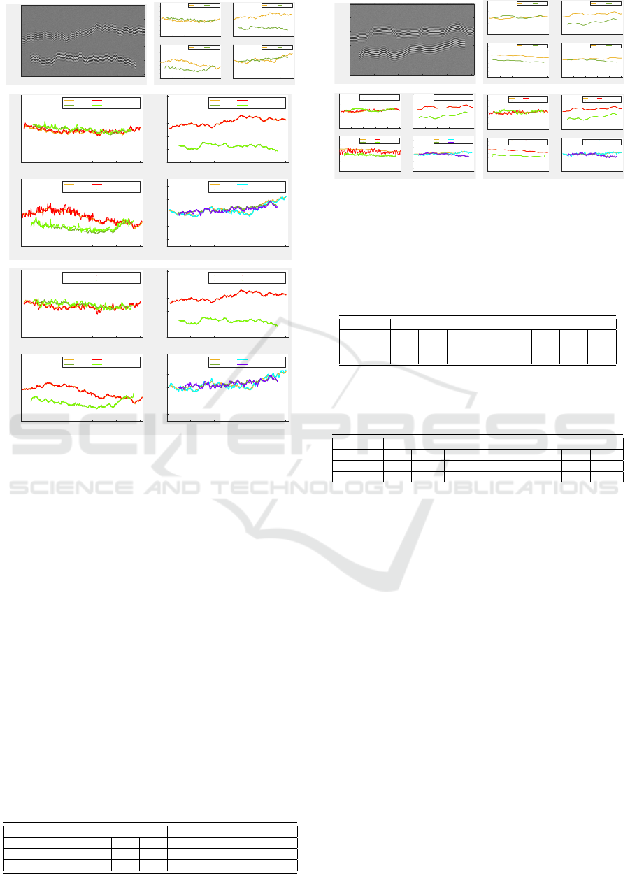
Figure 2: Image 1. (a): Synthetic interferometric signal;
(b): true trajectories (from top left to bottom right: variance,
surface, frequency, amplitude) ; (c): estimated trajectories
by TK algorithm; (d) estimated trajectories by TK-MCMC.
The value of R corresponds to a SNR fixed to
15 dB. For the parameters r
c
, r
a
, r
w
, r
ν
, TK-MCMC
method improves the estimated values relative to TK
method. The estimation of R is identical, since this
is based on the variance calculated in a homogeneous
area of the initial image. This estimated value there-
fore does not depend on the method chosen after-
ward. Table 2 shows the error rates (in percentage)
between the original trajectories and the estimated
trajectories, concerning the centers, amplitudes, vari-
ances and normalized pulsations. It is obvious regard-
ing to these results, that in the specific case of rougher
surfaces, TK-MCMC method noticeably improves the
error rates. Note that the estimation of the error re-
lated to the surfaces is particularly important, since
Table 2: Image 1 (Fig. 2): error rate between true and es-
timated trajectories for surfaces, amplitudes, variances and
frequencies for TK and MCMC algorithms.
Class 1 Class 2
c
k,n
a
k,n
σ
k,n
ν
k,n
c
k,n
a
k,n
σ
k,n
ν
k,n
TK % 0.76 1.36 1.93 2.91 0.38 1.58 1.59 3.65
MCMC % 0.02 1.13 1.25 0.37 1.4·10
−2
1.14 1.38 0.40
50 100 150 200 250
lateral axis x
50
100
150
200
250
optical axis z
0 50 100 150 200 250
Original frequencies
0.2
0.4
0.6
0.8
1
1.2
1.4
1.6
Class 1 Class 2
0 50 100 150 200 250
Original surfaces
0
50
100
150
200
250
Class 1 Class 2
0 50 100 150 200 250
Original amplitudes
15
20
25
30
35
Class 1 Class 2
0 50 100 150 200 250
Original variances
0.3
0.4
0.5
0.6
0.7
0.8
Class 1 Class 2
(a) (b)
0 50 100 150 200 250
Original and estimated frequencies
0.2
0.4
0.6
0.8
1
1.2
1.4
1.6
Class 1
Class 2
Estimated classe 1
Estimated class 2
0 50 100 150 200 250
Original and estimated surfaces
0
50
100
150
200
250
Class 1
Class 2
Estimated classe 1
Estimated class 2
0 50 100 150 200 250
Original and estimated amplitudes
15
20
25
30
35
Class 1
Class 2
Estimated classe 1
Estimated class 2
0 50 100 150 200 250
Original and estimated variances
0.3
0.4
0.5
0.6
0.7
0.8
Class 1
Class 2
Estimated classe 1
Estimated class 2
0 50 100 150 200 250
Original and estimated frequencies
0.2
0.4
0.6
0.8
1
1.2
1.4
1.6
Class 1
Class 2
Estimated classe 1
Estimated class 2
0 50 100 150 200 250
Original and estimated surfaces
0
50
100
150
200
250
Class 1
Class 2
Estimated classe 1
Estimated class 2
0 50 100 150 200 250
Original and estimated amplitudes
15
20
25
30
35
Class 1
Class 2
Estimated classe 1
Estimated class 2
0 50 100 150 200 250
Original and estimated variances
0.3
0.4
0.5
0.6
0.7
0.8
Class 1
Class 2
Estimated classe 1
Estimated class 2
(c) (d)
Figure 3: Image 2. (a): Synthetic interferometric signal;
(b): true trajectories (from top left to bottom right: variance,
surface, frequency, amplitude) ; (c): estimated trajectories
by TK algorithm; (d) estimated trajectories by TK-MCMC.
Table 3: Image 2 (Fig. 3): error rate between true and es-
timated trajectories for surfaces, amplitudes, variances and
frequencies for TK and MCMC algorithms.
Class 1 Class 2
c
k,n
a
k,n
σ
k,n
ν
k,n
c
k,n
a
k,n
σ
k,n
ν
k,n
TK % 0.09 2.10 1.44 7.84 0.06 0.77 1.35 2.88
MCMC % 0.01 1.71 1.59 0.21 0.01 1.63 1.49 0.25
Table 4: Image 3 (Fig. 4): error rate between true and es-
timated trajectories for surfaces, amplitudes, variances and
frequencies for C-TK and MCMC algorithms.
Class 1 Class 2
c
k,n
a
k,n
σ
k,n
ν
k,n
c
k,n
a
k,n
σ
k,n
ν
k,n
C-TK % 1.86 17.20 4.39 27.88 1.11 5.78 2.77 12.20
MCMC % 0.02 1.73 2.29 0.24 0.01 1.45 1.82 0.17
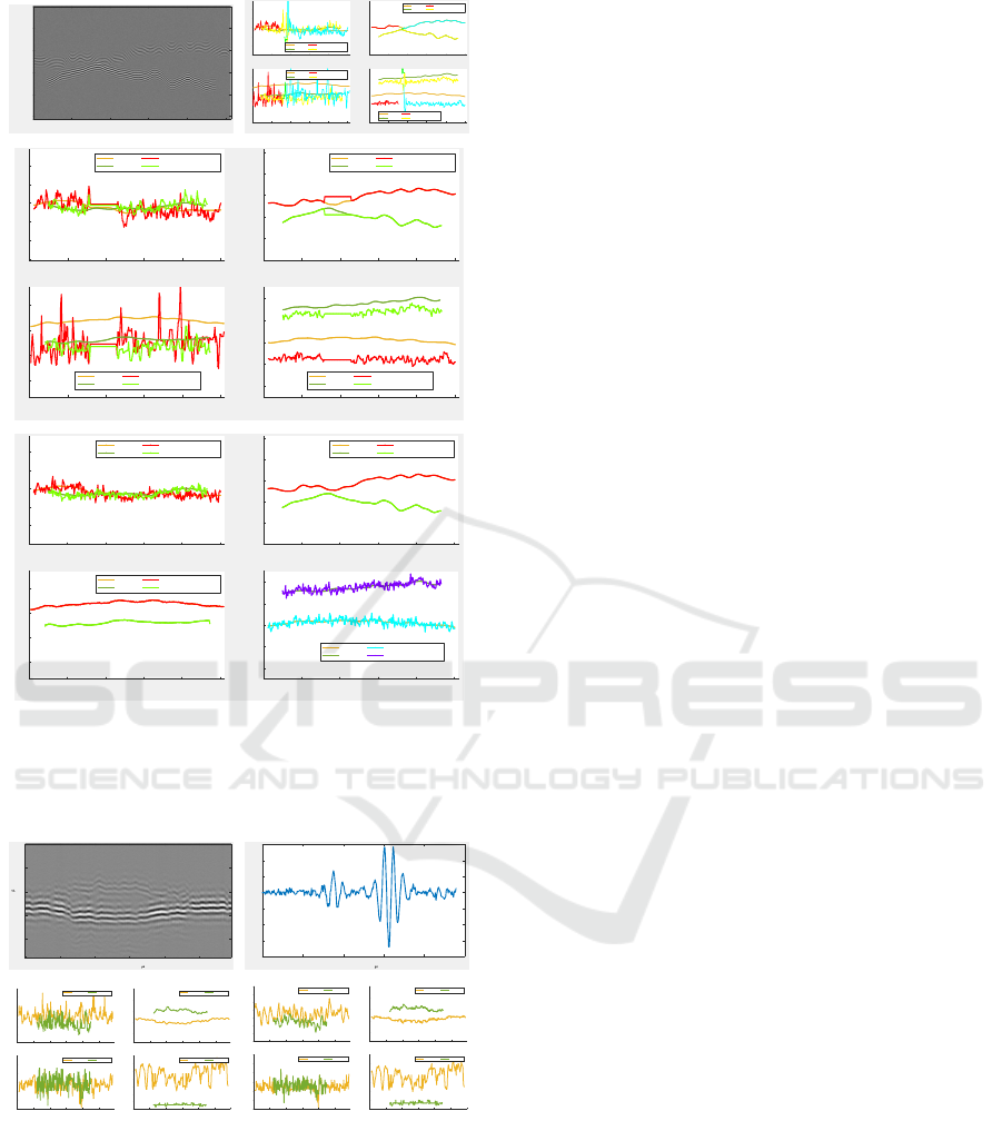
it indicates to the shape of surface material. Figure
3(a) represents two smooth surfaces (simulated us-
ing Markovian processes whose trajectories were then
smoothed by spline functions) and their estimation by
both methods (Fig. 3(c)-(d)). The error rates of the
corresponding trajectories are reported in Table 3.
Here again, we remark that TK-MCMC algorithm
significantly improves the calculation of the parame-
ters (especially the shape of the surfaces i.e., the tra-
jectories of the centers, as well as the estimated fre-
quencies), except for the variance. Figure 4(a) illus-
trates a situation where two surfaces are close in a
region of the interferometric data. Figure 4(b) rep-
resents the trajectories estimated by TK algorithm,
which fails to connect the surfaces, and introduces
parasitic classes.
Surface Extraction in Coherence Scanning Interferometry by Gauss-Markov Monte-Carlo Method and Teager-Kaiser Operator
399
50 100 150 200 250
lateral axis x
50
100
150
200
250
optical axis z
0 50 100 150 200 250
Original and estimated frequencies
0.5
1
1.5
2
Class 1
Class 2
Estimated classe 1
Estimated class 2
0 50 100 150 200 250
Original and estimated surfaces
0
50
100
150
200
250
Class 1
Class 2
Estimated classe 1
Estimated class 2
0 50 100 150 200 250
Original and estimated amplitudes
15
20
25
30
35
Class 1
Class 2
Estimated classe 1
Estimated class 2
0 50 100 150 200 250
Original and estimated variances
0.3
0.4
0.5
0.6
0.7
0.8
Class 1
Class 2
Estimated classe 1
Estimated class 2
(a) (b)
0 50 100 150 200 250
Original and estimated frequencies
0.5
1
1.5
2
Class 1
Class 2
Estimated classe 1
Estimated class 2
0 50 100 150 200 250
Original and estimated surfaces
0
50
100
150
200
250
Class 1
Class 2
Estimated classe 1
Estimated class 2
0 50 100 150 200 250
Original and estimated amplitudes
15
20
25
30
35
Class 1
Class 2
Estimated classe 1
Estimated class 2
0 50 100 150 200 250
Original and estimated variances
0.3
0.4
0.5
0.6
0.7
0.8
Class 1
Class 2
Estimated classe 1
Estimated class 2
(c)
0 50 100 150 200 250
Original and estimated frequencies
0.5
1
1.5
2
Class 1
Class 2
Estimated classe 1
Estimated class 2
0 50 100 150 200 250
Original and estimated surfaces
0
50
100
150
200
250
Class 1
Class 2
Estimated classe 1
Estimated class 2
0 50 100 150 200 250
Original and estimated amplitudes
15
20
25
30
35
Class 1
Class 2
Estimated classe 1
Estimated class 2
0 50 100 150 200 250
Original and estimated variances
0.3
0.4
0.5
0.6
0.7
0.8
Class 1
Class 2
Estimated classe 1
Estimated class 2
(d)
Figure 4: Image 3. (a): Synthetic interferometric signal;
(b): estimated trajectories by TK algorithm (surface, am-
plitude, variance, frequency); (c): corrected estimation by
close surfaces algorithm; (d) estimation by MCMC.
0 10 20 30 40 50
lateral axis x ( m)
0
5
10
15
20
optical axis z ( m)
0 5 10 15 20 25
optical axis ( m)
-80
-60
-40
-20
0
20
40
60
intensity
(a) (b)
0 10 20 30 40 50
Estimated frequencies (y-axis in MHz)
1.5
2
2.5
3
3.5
4
4.5
Class 1 Class 2
0 10 20 30 40 50
Estimated surfaces
0
5
10
15
20
Class 1 Class 2
0 10 20 30 40 50 60
Estimated amplitudes
0
20
40
60
80
100
120
140
Class 1 Class 2
0 10 20 30 40 50
Estimated variances
15
20
25
30
35
40
45
50
Class 1 Class 2
0 10 20 30 40 50
Estimated frequencies (y-axis in MHz)
1.5
2
2.5
3
3.5
4
4.5
Class 1 Class 2
0 10 20 30 40 50
Estimated surfaces
0
5
10
15
20
Class 1 Class 2
0 10 20 30 40 50 60
Estimated amplitudes
0
20
40
60
80
100
120
Class 1 Class 2
0 10 20 30 40 50
Estimated variances
15
20
25
30
35
40
45
50
Class 1 Class 2
(c) (d)
Figure 5: Image 5. (a): Real interferometric signal; (b):
profile along the optical axis; (c): estimated trajectories by
TK algorithm; (d) estimated trajectories by TK-MCMC.
We show in Figure 4(c) the efficiency of the
method stated above taking into account the close sur-
faces, so as to connect the surfaces, initializing vari-
ances, amplitudes and centers around the area of con-
nection, noted by C-TK algorithm. Finally, figure
4(d) illustrates the application of the MCMC method
following this initialization.
According to table 4 and error rates, its effective-
ness is clear. Finally figure 5 illustrates the applica-
tion of our method to a real interferometric signal. We
notice in particular that TK and TK-MCMC manage
to discriminate well the amplitudes corresponding to
the two respective surfaces, which are quite different
as shown in figures 5(b). By comparing figure 5(c)
and 5(d), TK-MCMC method better homogenizes the
values of the carrier frequencies, and more accurately
estimates the roughness of the involved surfaces.
7 CONCLUSION
In this article, we have introduced a new method for
automatic extraction of material surfaces, combining
two types of approaches: a TK nonlinear operator
and a Gauss-Markov model introducing a statistical
dependence between the surface neighboring points
based on four parameters which are able to character-
ize a fringe signal. This assumption notably makes
it possible to extract the homogeneity information
by means of the variance parameter. The parame-
ters of the Markovian model, after initialization us-
ing TKEO, have been estimated by a MCMC proce-
dure. In the presence of different layers of materi-
als, our method proposes an identification of these,
by assigning the points according to a distance cri-
terion. On the other hand, we have studied the case
of close surfaces, for which an initialization by the
TK algorithm alone is insufficient. In the areas where
the points of close surfaces are badly estimated, an
algorithm makes it possible to extend the trajectories
of these surfaces which are located nearby them. We
have numerically illustrated the performance of our
method on synthetic and real images, showing an abil-
ity to match the roughness of the surfaces. A possible
extension of our algorithm could concern on the one
hand, upstream an improvement of the initialization
by means of a more adapted TK algorithm (for exam-
ple a higher order one or by using one the new algo-
rithms as proposed in (Pr
´
eaux and Boudraa, 2022)).
And also an exploitation of the lateral information
provided by the neighbored xz sections within a data
cube. This would be particularly useful to improve the
identification of close surfaces. The complexification
of the Markovian model by introducing for instance
correlated noise, represents another challenge.
ICPRAM 2024 - 13th International Conference on Pattern Recognition Applications and Methods
400

REFERENCES
Boudraa, A.-O., Cexus, J.-C., Groussat, M., and Brunagel,
P. (2008). An energy-based similarity measure for
time series. EURASIP Journal on Advances in Sig-
nal Processing, 2008:1–8.
Boudraa, A.-O. and Salzenstein, F. (2018). Teager–kaiser
energy methods for signal and image analysis: A re-
view. Digital Signal Processing, 78:338–375.
Boudraa, A.-O., Salzenstein, F., and Cexus, J.-C. (2005).
Two-dimensional continuous higher-order energy op-
erators. Optical Engineering, 44(11):117001–117001.
Chim, S. S. and Kino, G. S. (1990). Correlation microscope.
Optics Letters, 15(10):579–581.
de Groot, P., de Lega, X. C., Kramer, J., and Turzhit-
sky, M. (2002). Determination of fringe order in
white-light interference microscopy. Applied optics,
41(22):4571–4578.
de Groot, P. and Deck, L. (1993). Three-dimensional imag-
ing by sub-nyquist sampling of white-light interfero-
grams. Optics Letters, 18(17):1462–1464.
Gianto, G., Salzenstein, F., and Montgomery, P. (2016).
Comparison of envelope detection techniques in co-
herence scanning interferometry. Applied Optics,
55(24):6763–6774.
Guo, T., Ma, L., Chen, J., Fu, X., and Hu, X. (2011).
Microelectromechanical systems surface characteri-
zation based on white light phase shifting interferom-
etry. Optical Engineering, 50(5):053606–053606.
Gurov, I., Ermolaeva, E., and Zakharov, A. (2004). Analysis
of low-coherence interference fringes by the kalman
filtering method. Journal of the Optical Society of
America A, 21(2):242–251.
Gurov, I. and Volynsky, M. (2012). Interference fringe anal-
ysis based on recurrence computational algorithms.
Optics and Lasers in Engineering, 50(4):514–521.
Hissmann, M. and Hamprecht, F. A. (2005). Bayesian sur-
face estimation for white light interferometry. Optical
Engineering, 44(1):015601–015601.
Kemao, Q. (2004). Windowed fourier transform for fringe
pattern analysis. Applied Optics, 43(13):2695–2702.
Kroese, D. P., Taimre, T., and Botev, Z. I. (2013). Handbook
of Monte-Carlo Methods. John Wiley & Sons.
Larkin, K. G. (1996). Efficient nonlinear algorithm for en-
velope detection in white light interferometry. Journal
of the Optical Society of America A, 13(4):832–843.
Larkin, K. G. (2005). Uniform estimation of orientation
using local and nonlocal 2-d energy operators. Optics
Express, 13(20):8097–8121.
Li, M., Quan, C., and Tay, C. (2008). Continuous wavelet
transform for micro-component profile measurement
using vertical scanning interferometry. Optics &
Laser Technology, 40(7):920–929.
Ma, S., Quan, C., Zhu, R., Tay, C., Chen, L., and Gao,
Z. (2011). Micro-profile measurement based on win-
dowed Fourier transform in white-light scanning in-
terferometry. Optics Communications, 284(10):2488–
2493.
Maragos, P. and Bovik, A. C. (1995). Image demodulation
using multidimensional energy separation. Journal of
the Optical Society of America A, 12(9):1867–1876.
Maragos, P., Kaiser, J. F., and Quatieri, T. F. (1993). Energy
separation in signal modulations with application to
speech analysis. IEEE Transactions on Signal Pro-
cessing, 41(10):3024–3051.
Maragos, P. and Potamianos, A. (1995). Higher order dif-
ferential energy operators. IEEE Signal Processing
Letters, 2(8):152–154.
Mazet, V., Faisan, S., Awali, S., Gaveau, M.-A., and Pois-
son, L. (2015). Unsupervised joint decomposition of
a spectroscopic signal sequence. Signal Processing,
109:193–205.
Niu, H., Quan, C., and Tay, C. (2009). Phase re-
trieval of speckle fringe pattern with carriers using 2d
wavelet transform. Optics and Lasers in Engineering,
47(12):1334–1339.
O’Mahony, C., Hill, M., Brunet, M., Duane, R., and Math-
ewson, A. (2003). Characterization of micromechan-
ical structures using white-light interferometry. Mea-
surement Science and Technology, 14(10):1807.
Pavli
ˇ
cek, P. and Michalek, V. (2012). White-light interfer-
ometryenvelope detection by hilbert transform and in-
fluence of noise. Optics and Lasers in Engineering,
50(8):1063–1068.
Pr
´
eaux, Y. and Boudraa, A.-O. (2022). Discr
´
etisation de
l’op
´
erateur d’
´
energie de teager-kaiser revisit
´
ee. In
Colloque Grestsi.
Pr
´
eaux, Y., Boudraa, A.-O., and Larkin, K. G. (2022). On
the positivity of teager-kaiser’s energy operator. Sig-
nal Processing, 201:108702.
Salzenstein, F., Boudraa, A.-O., and Cexus, J.-C. (2007).
Generalized higher-order nonlinear energy opera-
tors. Journal of the Optical Society of America A,
24(12):3717–3727.
Salzenstein, F., Boudraa, A.-O., and Chonavel, T. (2013).
A new class of multi-dimensional teager-kaiser and
higher order operators based on directional deriva-
tives. Multidimensional Systems and Signal Process-
ing, 24:543–572.
Salzenstein, F., Montgomery, P., and Boudraa, A.-O.
(2014). Local frequency and envelope estimation by
teager-kaiser energy operators in white-light scanning
interferometry. Optics Express, 22(15):18325–18334.
Sandoz, P. (1997). Wavelet transform as a processing
tool in white-light interferometry. Optics Letters,
22(14):1065–1067.
Wu, D. and Boyer, K. L. (2011). Markov random field based
phase demodulation of interferometric images. Com-
puter Vision and Image Understanding, 115(6):759–
770.
Zhu, P. and Wang, K. (2012). Single-shot two-
dimensional surface measurement based on spectrally
resolved white-light interferometry. Applied optics,
51(21):4971–4975.
Zou, W., Zhu, L., Wang, W., and Chen, C. (2016). Bayesian
denoising of white light interference signal in rough
surface measurement. In MATEC Web of Conferences,
volume 61, page 01002. EDP Sciences.
Surface Extraction in Coherence Scanning Interferometry by Gauss-Markov Monte-Carlo Method and Teager-Kaiser Operator
401
