Introducing Reduced-Width QNNs, an AI-Inspired

Ansatz Design Pattern

Jonas Stein

1,2,∗ a

, Tobias Rohe

1,∗

, Francesco Nappi

, Julian Hager

, David Bucher

2 b

Maximilian Zorn

1 c

, Michael Kölle

1 d

and Claudia Linnhoff-Popien

1 e

Mobile and Distributed Systems Group, LMU Munich, Germany

Aqarios GmbH, Germany

ﬁ

Keywords:

Quantum Computing, Variational Quantum Circuits, Circuit Optimization, Variational Quantum Eigensolver.

Abstract:

Variational Quantum Algorithms are one of the most promising candidates to yield the ﬁrst industrially relevant

quantum advantage. Being capable of arbitrary function approximation, they are often referred to as Quantum

Neural Networks (QNNs) when being used in analog settings as classical Artiﬁcial Neural Networks (ANNs).

Similar to the early stages of classical machine learning, known schemes for efﬁcient architectures of these

networks are scarce. Exploring beyond existing design patterns, we propose a reduced-width circuit ansatz

design, which is motivated by recent results gained in the analysis of dropout regularization in QNNs. More

precisely, this exploits the insight, that the gates of overparameterized QNNs can be pruned substantially

until their expressibility decreases. The results of our case study show, that the proposed design pattern can

signiﬁcantly reduce training time while maintaining the same result quality as the standard "full-width" design

in the presence of noise. We thus argue, that quantum architecture search should not blindly follow the classical

overparameterization trend.

1 INTRODUCTION

A central goal of current quantum computing re-

search is achieving an industrially relevant quan-

tum advantage. As immense computational require-

ments of known quantum algorithms enabling prov-

able speedups exceed prevailing hardware capabilities

in the present NISQ era, less demanding approaches

like Quantum Neural Networks (QNNs) are of great

interest, especially as they have already shown very

promising results towards a possible quantum advan-

tage (Abbas et al., 2021). QNNs closely resem-

ble classical Artiﬁcial Neural Networks (ANNs), as

they are composed of concatenated, parameterized

functions capable of approximating arbitrary func-

tions (Mitarai et al., 2018). The core difference be-

tween QNNs and ANNs is the dimensionality of the

underlying vector space, which is exponentially larger

https://orcid.org/0000-0001-5727-9151

https://orcid.org/0009-0002-0764-9606

https://orcid.org/0009-0006-2750-7495

https://orcid.org/0000-0002-8472-9944

https://orcid.org/0000-0001-6284-9286

∗

These authors contributed equally.

in the former with respect to the space requirements

in qubits/neurons (Mitarai et al., 2018).

A key advantage of QNNs compared to estab-

lished quantum algorithms like those of (Shor, 1994)

or (Grover, 1996) is their ﬂexibility towards respect-

ing restricted hardware capabilities. More precisely,

QNNs can be shaped to ﬁt a maximal width and

depth of the circuit to be executed on the QPU and

can thus minimize errors caused, e.g., by decoher-

ence. Analogous to the historical progress on ANNs,

where many useful and performant network architec-

tures and design patterns emerged, recent literature

on QNNs explores productive quantum circuit de-

sign patterns (Cerezo et al., 2021a; Sim et al., 2019a;

Schuld et al., 2021; Havlí

cek et al., 2019). Similar to

ANNs, these techniques are used to ﬁnd a sufﬁciently

good trade-off between expressibility and trainability.

In classical machine learning, this problem is pre-

dominantly solved by utilizing heavily overparame-

terized models and regularization techniques to fa-

cilitate efﬁcient trainability. A particularly powerful

regularization technique is dropout, in which parts

of the model are randomly deleted for each training

step. Among other effects, this introduces noise to

the network architecture and therefore hinders overﬁt-

Stein, J., Rohe, T., Nappi, F., Hager, J., Bucher, D., Zorn, M., Kölle, M. and Linnhoff-Popien, C.

Introducing Reduced-Width QNNs, an AI-Inspired Ansatz Design Pattern.

DOI: 10.5220/0012449800003636

Paper published under CC license (CC BY-NC-ND 4.0)

In Proceedings of the 16th International Conference on Agents and Artiﬁcial Intelligence (ICAART 2024) - Volume 3, pages 1127-1134

ISBN: 978-989-758-680-4; ISSN: 2184-433X

1127

ting (Srivastava et al., 2014). Meanwhile, even though

research on regularization techniques for QNNs is

still in its early stages, dropout has also shown ﬁrst

promising results (Scala et al., 2023; Kobayashi et al.,

2022). Analyses on instances of overparameterized

QNNs in (Scala et al., 2023) show no reduction of ex-

pressibility in the presence of substantial gate prun-

ing. In this article, we use these insights as inspira-

tion for an ansatz design pattern, that directly employs

a gate-pruned version of overparameterized QNNs.

This is explicitly not targeted towards substituting

dropout, but meant as an exploration of the neces-

sity of the standard full-width layer design in the ﬁrst

place.

To test the effectiveness of our approach, we eval-

uate QNNs of a ﬁxed circuit architecture before and

after pruning. Our main contributions in this paper

can thus be summarized as the following:

• We propose a novel, AI-inspired QNN design pat-

tern, that can notably also be applied as a pruning

technique for existent QNNs.

• We conduct an empirical case study of this design

pattern for the maximum cut optimization prob-

lem in a noisy environment.

2 BACKGROUND

In the following, we describe the core algorithms and

techniques employed in our methodology. We show

how QNNs can be utilized to solve speciﬁc optimiza-

tion problems like the maximum cut problem as part

of a Variational Quantum Eigensolver (VQE).

2.1 Quantum Neural Networks

In current literature, the term Quantum Neural Net-

work is predominantly used to describe a Parameter-

ized Quantum Circuit (PQC) utilized for tasks typ-

ical for classical Artiﬁcial Neural Networks. Al-

though the terminology suggests a close similarity be-

tween QNNs and ANNs, there exist signiﬁcant dif-

ferences. A core distinction is that QNNs do not

consist of individual neurons, instead they are com-

prised of qubits, whose states can be changed using

(parameterized) quantum gates, that can involve inter-

actions with other qubits. Despite the substantial dif-

ferences between ANNs and QNNs, there also exist

strong commonalities, foremost the shared capability

of universal function approximation, i.e., ANNs and

QNNs can both be described as parameterized func-

tions, that can approximate arbitrary functions un-

der certain conditions (Schuld et al., 2021). More-

over, by representing QNNs and feedforward ANNs

Output

Hidden

Input

Figure 1: Example network architecture of the encoder in

an autoencoder.

as mathematical functions, we can observe clear sim-

ilarities. A feedforward neural network is mathe-

matically represented by concatenations of typically

non-linear activation functions for all neurons in each

layer (Schmidhuber, 2015). In contrast, QNNs typ-

ically model concatenations of linear layers with a

single non-linear layer at the end, which is respon-

sible for the measurement, i.e., generating a classical

output (Mitarai et al., 2018). For examples of feedfor-

ward ANNs and QNNs, see Figs. 1 and 2.

Mathematically, the ﬁnal state of a QNN com-

posed of n ∈ qubits can be formalized as denoted

in Eq. 1

. In this formalization, we started in the stan-

dard initial state |0⟩

⊗n

and subsequently applied a pa-

rameterized unitary operation U (θ), with parameters

θ ∈

, where m ∈ denotes the number of parame-

ters. In practice, U is predominantly comprised of pa-

rameterized single-qubit and two-qubit gates to match

native gate sets of existing quantum computers.

|ψ(θ)⟩

= U (θ) |0⟩

⊗n

(1)

To extract classical information from the ﬁnal

state of the QNN, we typically measure each qubit

|ψ

⟩ in the computational basis

{

|0⟩,|1⟩

}

using the

measurement operator M = I

i−1

⊗ σ

⊗ I

n−i

, where

denotes the Pauli-Z operator. These measure-

ments yield a probability distribution over bitstrings

|x⟩ ∈

representing the output of the quantum cir-

cuit, where |x⟩ occurs at probability

⟨x | ψ (θ)⟩

Having presented an overview of the circuit com-

ponents of a QNN, we now address parameter train-

ing approaches. Analogous to ANNs, two main types

of parameter optimization approaches exist: gradient-

based and derivative-free methods (Mitarai et al.,

2018). While QNNs can be trained with essentially

the same techniques as ANNs, i.e., using approaches

like gradient descent, genetic algorithms, and others,

known gradient computations for QNNs are funda-

mentally more expensive. Using backpropagation, the

gradient in feedforward ANNs can be calculated as

This formalization explicitly disregards intermediate

measurements, in-line with predominant literature.

ICAART 2024 - 16th International Conference on Agents and Artiﬁcial Intelligence

1128

fast as a forward pass of the ANN, whereas all known

quantum gradient computations need O (m) execu-

tions of the QNN, where m ∈ denotes the num-

ber of parameters (Mitarai et al., 2018; Schuld et al.,

2019). The standard method to calculate the gradi-

ent of a parameterized quantum circuit is the param-

eter shift rule, which is used to calculate each par-

tial derivative

∂

/∂θ

U (θ)|0⟩

⊗n

based on Eq. 2, given

that all parameters are enclosed in single qubit gates

and θ

= (θ

,..., θ

i−1

,θ

/2,θ

i+1

,..., θ

) (Mitarai

et al., 2018; Schuld et al., 2019).

∂

∂θ

U (θ)|0⟩

⊗n

U (θ

)|0⟩

⊗n

−U (θ

−

)|0⟩

⊗n

(2)

Given this linear runtime increase in the gradient

computation for QNNs, achieving better solution

quality or a quick convergence to sufﬁciently good

parameters is essential for QNNs.

2.2 The Maximum Cut Problem in

Quantum Optimization

The maximum cut problem, is an NP-hard combinato-

rial optimization problem with the objective of parti-

tioning the nodes v

∈ V of a given graph G (V,E) into

two complementary sets A

∪B = V such that number

of edges between A and B is maximal. Encoding a

partitioning via a binary vector s ∈

{

−1,1

}

, where

and s

= 1 ⇔ v

∈ A and s

= −1 ⇔ v

∈ B, the

search for the optimal partition can be formulated as

shown in Eq. 3 (Lucas, 2014). This formulation nat-

urally evolves after observing that

(

1−s

)

/2 ∈

{

0,1

}

equals one iff the edge (v

) ∈ E connects A and B.

argmin

s∈

{

−1,1

}

∑

)∈E

(3)

We have chosen this ±1 encoding of the solution, as

it can directly be transformed into a quantum Hamil-

tonian

H that represents the solution space of this op-

timization problem, which is the standard approach

in quantum optimization exploiting that Ising Hamil-

tonians are isomorphic to the NP-hard QUBO. For

this, we merely need to substitute s

using the map

7→ σ

= I

⊗i−1

⊗ σ

⊗ I

⊗n−i

, where I denotes the

two dimensional identity matrix. Therefore, we can

deﬁne

∑

(

)

∈E

Switching to a 0/1 encoding, i.e., x ∈

{

0,1

}

with

= 0 ⇔ v

∈ A and x

= 1 ⇔ v

∈ B,

H can be un-

derstood as a mapping between solutions x and the

value of the objective function. More speciﬁcally, its

eigenvalues for a given eigenvector |x⟩ are the values

of the objective function, where x represents the 0/1

encoding of the solution.

2.3 The Variational Quantum

Eigensolver

The Variational Quantum Eigensolver (VQE) is an

algorithm targeted towards ﬁnding the ground state

of a given Hamiltonian

H using the variational

method (Peruzzo et al., 2014). The term varia-

tional method describes the process of making small

changes to a function f to ﬁnd minima or maxima

of a given function g (Lanczos, 2012). In the case

of the VQE, f : θ 7→ U (θ)|0⟩

⊗n

describes a param-

eterized quantum circuit yielding the state |ψ(θ)⟩

U (θ)|0⟩

⊗n

which represents a guess of the argmin of

the function g : |ϕ⟩ 7→ ⟨ϕ|

H |ϕ⟩. More speciﬁcally, the

VQE uses parameter training techniques on the given

ansatz U (θ) to generate an output state |ψ (θ)⟩ that

approximates the ground state of

For our purposes, i.e., solving an optimization

problem, we need to (1) deﬁne a Hamiltonian en-

coding our objective function and (2) select a suit-

able ansatz in order to use the VQE algorithm. While

we can use the procedure exempliﬁed in Sec. 2.2 to

deﬁne a Hamiltonian

H, the selection of the ansatz

and thus a circuit architecture is not thoroughly under-

stood yet. Although literature on automatized quan-

tum architecture search tools is emerging (Du et al.,

2022), most ansätze are designed based on empiric

experience (Sim et al., 2019b).

3 RELATED WORK

A suitable circuit design in QNNs is essential for

achieving good results in variational quantum com-

puting and is actively researched in literature (Sim

et al., 2019b). While some design patterns like a lay-

erwise circuit structure with alternating single qubit

rotations and entanglement gates, have become stan-

dard practice (Sim et al., 2019b), the list of estab-

lished circuit elements still is considerably smaller

than that in classical neural networks. A central

problem when trying to design ansätze is the trade-

off between expressibility and trainablity. Reason-

ably complex models demand for expressive circuits,

which in turn can quickly lead to the problem of bar-

ren plateaus, a trainability issue where the proba-

bility that the optimizer-gradient becomes exponen-

tially small is directly dependent on the number of

qubits (McClean et al., 2018). Moreover, barren

plateaus are found to be dependent on the choice of

the cost function itself (Cerezo et al., 2021b) as well

as the number of parameters to optimize simultane-

ously (Skolik et al., 2021).

Classical deep learning faced a similar problem

Introducing Reduced-Width QNNs, an AI-Inspired Ansatz Design Pattern

1129

in vanishing gradients, e.g., for recurrent neural net-

works (Hochreiter, 1998), which eventually lead to

the adoption of more specialized network architec-

tures like the long short-term memory (LSTM) net-

works (Hochreiter and Schmidhuber, 1997) for se-

quence processing. Similarly, the current trend of

improving variational architectures focuses on opti-

mizing the designs of quantum circuit ansätze, e.g.,

via optimization procedures starting from randomized

circuits (Fösel et al., 2021). In this context, our work

shows that pruning gates of the standard full-width

circuit architecture can substantially increase train-

ability while retaining the same solution quality.

4 METHODOLOGY

In the subsequent sections, we describe our reduced-

width ansatz design pattern in two different variants

as pruned versions of a baseline ansatz. Concluding

our methodology, we describe our approach to param-

eter training and problem instance generation.

4.1 Full-Width Design

In the following, we introduce the design of our base-

line ansatz, which we coin full-width design. We

choose a very simple circuit architecture consisting of

BasicEntanglerLayers

, as it resembles the most

basic circuit architecture and is ubiquitously used for

constructing variational quantum circuits in quantum

machine learning.

More speciﬁcally, this baseline circuit is con-

structed of two components. The ﬁrst is a sequence of

parameterized gates, i.e., a Pauli-X, a Pauli-Z and an-

other Pauli-X rotation, applied to each qubit, allowing

for the implementation of arbitrary single qubit oper-

ations. The second is a circular CNOT-entanglement,

i.e., CNOTs applied to all neighboring qubit pairs, us-

ing the maximum width of the circuit. We combine

these single- and two-qubit gate components into a

single layer, where every circuit is composed of four

such layers to analyse scaling behavior. The entire

circuit with all its layers is illustrated in Fig. 2. In

the following sections, we will refer to this circuit de-

sign as the full-width circuit or full-width design, as it

uses the same maximum width throughout all layers.

All the circuits utilized in this study are derived from

this full-width circuit, where variations are introduced

through the removal of gates.

For details and the implementation, see

https://docs.pennylane.ai/en/stable/code/api/pennylane.

BasicEntanglerLayers.html.

4.2 Reduced-Width Design

In this section, we introduce two different approaches

that reduce the width of a given ansatz by pruning

gates in a layerwise manner. The ﬁrst approach works

analog to the dropout employed in (Scala et al., 2023)

and randomly prunes the a ﬁxed number of gates from

the circuit (for reference, see Fig. 3). To test how the

structure of the employed pruning affects the perfor-

mance, we propose a second approach, which gradu-

ally increases the number of pruned gates for subse-

quent layers (for reference, see Fig. 4).

Starting with the detailed discussion of the sec-

ond approach, we review a key result of (Scala et al.,

2023), which states that the deeper the circuits, the

more gates can be pruned before effectively reducing

the expressibility. This is very sensible, as their re-

sults on the effectiveness of pruning are conditioned

on present overparameterization, which only occurs

for reasonably deep QNNs. Furthermore, we argue,

when entanglement between the qubits is sufﬁciently

high (i.e., in general after some ansatz layers), every

gate executed on a subset of these qubits intrinsically

also acts on all qubits, as they must be regarded as one

system. A well-known example in which exactly this

happens, is the ancilla quantum encoding as part of

the quantum algorithm for solving linear systems of

equations (Harrow et al., 2009; Stougiannidis et al.,

2023), in which controlled rotations on a single an-

cilla qubit substantially change the state of an entire

qubit register.

In our implementation, we reduce the circuit

width in every layer by a magnitude of two in a sym-

metric manner. This implies that the outermost qubits

manipulated in the previous layer are no longer al-

tered directly in the appended layer. This reduction

applies to both single- and two-qubit gates. Conse-

quently, the circular entanglement is applied solely to

the remaining inner qubits, so that gates are not only

deleted, but also reconnected. A visualization of our

reducing-width ansatz can be found in Fig. 4.

The number of reduced single- and two-qubits

gates is dependent on the number of qubits n, the

number of layers l, and the magnitude by which the

circuit width is reduced per layer m. Further, we

have to distinguish between the reduction in one-qubit

gates

∑

i=1

(i − 1)3m, and the reduction in two-qubit

gates

∑

i=1

(i − 1)m. The proposed reduction is nat-

urally restricted by the number of qubits in the cir-

cuit, i.e., (l − 1)m < n must be satisﬁed, so that the

reduction can be conducted when starting from the

full-width circuit.

In our case (i.e., using eight qubits, four ansatz

layers, and a reduction of the circuit width per layer

ICAART 2024 - 16th International Conference on Agents and Artiﬁcial Intelligence

1130

(θ

) R

(θ

) R

(θ

)

•

(θ

) R

(θ

) R

(θ

)

•

(θ

) R

(θ

) R

(θ

)

•

(θ

) R

(θ

) R

(θ

)

•

(θ

) R

(θ

) R

(θ

)

•

(θ

) R

(θ

) R

(θ

)

•

(θ

) R

(θ

) R

(θ

)

•

(θ

) R

(θ

) R

(θ

)

•

(θ

) R

(θ

) R

(θ

)

•

(θ

) R

(θ

) R

(θ

)

•

(θ

) R

(θ

) R

(θ

)

•

(θ

) R

(θ

) R

(θ

)

•

(θ

) R

(θ

) R

(θ

)

•

(θ

) R

(θ

) R

(θ

)

•

(θ

) R

(θ

) R

(θ

)

•

(θ

) R

(θ

) R

(θ

)

•

(θ

) R

(θ

) R

(θ

)

•

(θ

) R

(θ

) R

(θ

)

•

(θ

) R

(θ

) R

(θ

)

•

(θ

) R

(θ

) R

(θ

)

•

(θ

) R

(θ

) R

(θ

)

•

(θ

) R

(θ

) R

(θ

)

•

(θ

) R

(θ

) R

(θ

)

•

(θ

) R

(θ

) R

(θ

)

•

(θ

) R

(θ

) R

(θ

)

•

(θ

) R

(θ

) R

(θ

)

•

(θ

) R

(θ

) R

(θ

)

•

(θ

) R

(θ

) R

(θ

)

•

(θ

) R

(θ

) R

(θ

)

•

(θ

) R

(θ

) R

(θ

)

•

(θ

) R

(θ

) R

(θ

)

•

(θ

) R

(θ

) R

(θ

)

•

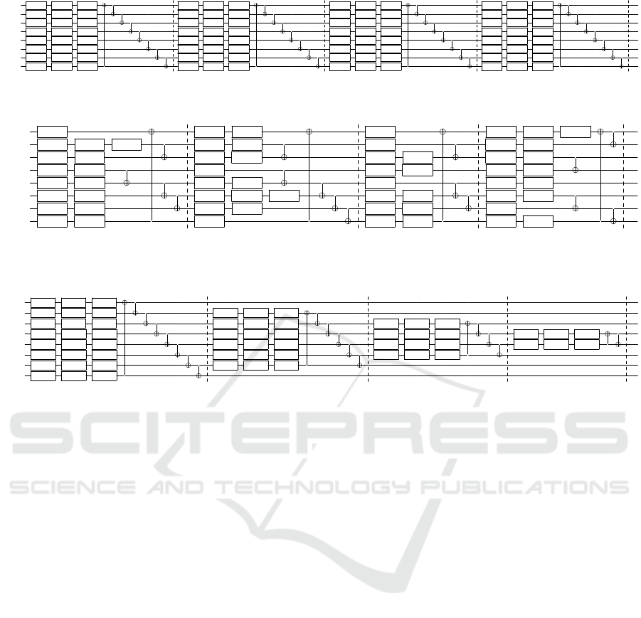
Figure 2: The full-width design in which gates are applied over the full width of the circuit throughout all layers. The circuit

is displayed with four layers, in-line with its conﬁguration in our evaluation.

(θ

) R

(θ

) R

(θ

) R

(θ

) R

(θ

) R

(θ

) R

(θ

)

•

(θ

) R

(θ

) R

(θ

)

•

(θ

) R

(θ

)

•

(θ

)

•

(θ

) R

(θ

)

(θ

) R

(θ

) R

(θ

) R

(θ

) R

(θ

) R

(θ

) R

(θ

) R

(θ

)

•

(θ

) R

(θ

)

•

(θ

)

•

(θ

) R

(θ

) R

(θ

) R

(θ

)

(θ

) R

(θ

)

•

(θ

) R

(θ

)

•

(θ

)

•

(θ

) R

(θ

)

(θ

) R

(θ

)

•

(θ

) R

(θ

) R

(θ

)

•

(θ

) R

(θ

)

•

(θ

) R

(θ

)

•

(θ

) R

(θ

) R

(θ

) R

(θ

)

•

(θ

) R

(θ

) R

(θ

)

•

(θ

) R

(θ

)

•

(θ

)

•

(θ

) R

(θ

)

•

(θ

) R

(θ

)

•

Figure 3: The random-width design in which a speciﬁc number of gates are deleted from the full-width design at random

positions. The number of gates removed gates equals the number of removed gates in the reducing-width circuit. The circuit

is displayed with four layers, in-line with its conﬁguration in our evaluation.

(θ

) R

(θ

) R

(θ

)

•

(θ

) R

(θ

) R

(θ

)

•

(θ

) R

(θ

) R

(θ

)

•

(θ

) R

(θ

) R

(θ

)

•

(θ

) R

(θ

) R

(θ

)

•

(θ

) R

(θ

) R

(θ

)

•

(θ

) R

(θ

) R

(θ

)

•

(θ

) R

(θ

) R

(θ

)

•

(θ

) R

(θ

) R

(θ

)

•

(θ

) R

(θ

) R

(θ

)

•

(θ

) R

(θ

) R

(θ

)

•

(θ

) R

(θ

) R

(θ

)

•

(θ

) R

(θ

) R

(θ

)

•

(θ

) R

(θ

) R

(θ

)

•

(θ

) R

(θ

) R

(θ

)

•

(θ

) R

(θ

) R

(θ

)

•

(θ

) R

(θ

) R

(θ

)

•

(θ

) R

(θ

) R

(θ

)

•

(θ

) R

(θ

) R

(θ

)

•

(θ

) R

(θ

) R

(θ

)

•

Figure 4: The reducing-width design in which the width is reduced from layer to layer by a magnitude of two. With this

design approach, we prune the circuit to a version which uses much fewer gates. The circuit is displayed with four layers,

in-line with its conﬁguration in our evaluation.

of two in magnitude), we reduce the number of one-

qubit gates by 36, and the number of two-qubit gates

by 12. Respectively, this corresponds to a reduction

of one-qubit gates by 37.5%, and a 50% reduction for

two-qubit gates. Beside the hypothesized positive ef-

fects that a reduction of the number of gates has on

the parameter optimization process, the proposed cir-

cuit design is naturally also more noise tolerant. More

speciﬁcally, the reduced number of gates and conse-

quently the lower circuit depth reduce the total noise

accumulated from imperfect gate ﬁdelities and deco-

herence (Hashim et al., 2023). We therefore expect

our approach to be the most beneﬁcial in a noisy en-

vironment.

As stated in the beginning of this section, we also

introduce the so called random-width design. Here,

we prune the same number and the same kind of gates

from the full-width design as in the reducing-width

approach. However, instead of removing these gates

in a systematic way, as done in the reducing-width

design, we randomly determine the gates for removal.

Therefore, the number and kind of gates compared

to the reducing-width design stays the same, but the

sequence and position of the gates differ. An exem-

plary circuit resulting from the random-width design

is shown in Fig. 3. To achieve statistical relevance in

the structure of the pruned gates, the results of three

different prunings are averaged over each problem in-

stance in the evaluation.

4.3 Training Method

Aiming for a test case in which our approach can

show its full potential (see Sec. 4.2), we decide

to restrict our evaluation to a noisy environment.

Therefore, we employ layerwise learning, which is a

method speciﬁcally targeted at coping with noise dur-

ing the training and has been shown to increase re-

sult quality signiﬁcantly in many cases (Skolik et al.,

2021). A small prestudy also shows that this is the

case for our setup. The training conceptually starts

with the ﬁrst layer of the respective circuit individu-

ally, i.e., without any other layers present in the cir-

cuit. Subsequently, the parameterized gates get ini-

tialized with zeroes to approximate an identity layer

similar to the approach proposed in (Liu et al., 2022)

and the parameter training is started. For the train-

ing process, we use the COBYLA optimizer (Pow-

ell, 1994), where the maximum number of iterations

is set to 300 to allow for the learning curve to con-

verge sufﬁciently, according to empirical pretests con-

ducted for this study. After the training of the ﬁrst

Introducing Reduced-Width QNNs, an AI-Inspired Ansatz Design Pattern

1131

layer is completed, the trained parameters get saved,

and a new quantum circuit is constructed. The new

circuit now implements two layers and re-uses the

previously trained and saved parameters for the ini-

tialization of the ﬁrst layer. The parameters of the

gates added in the next layer of the circuit are initial-

ized with zero, while the subsequent training-process

only trains the newly added layer of the respective

circuit. This training method now repeats itself un-

til all four layers are implemented and trained. This

training approach therefore aims at improving on ev-

ery previously achieved solution iteratively, similar to

techniques like reverse annealing.

4.4 Problem Instance Generation

To evaluate the performance of the three different de-

sign approaches, we solve the maximum cut prob-

lem for 50 randomly generated 8-node Erd

os-Rényi

graphs (Erd

os and Rényi, 1959) using a VQE setup

with the respective circuit design as the ansatz. These

graphs are generated in a random manner, where the

number of nodes, as well as the probability that an

edges exists between each pair of nodes, are given

as input. We use eight nodes to match the qubit

count and choose an edge probability of 50% to

yield reasonably realistic problem instances, analo-

gous to (Martiel et al., 2021).

5 EVALUATION

Our experiments are conducted with the three differ-

ent ansätze shown in Figs. 2, 3 and 4 aiming to solve

50 maximum cut problem instances using a VQE

approach and layerwise learning. As motivated in

Sec. 4.2, we employ depolarizing noise effects in our

circuit simulations: The one-qubit and two-qubit gate

error rate were both set to 1%, which roughly coin-

cides with the gate ﬁdelities of recent IBM QPUs. To

facilitate these comparatively compute intensive cir-

cuit simulations, we run our experiments on an Atos

Quantum Learning Machine (QLM).

In the following two sections, we investigate the

runtime and result quality of the proposed reduced-

width ansatz design pattern. To facilitate a basic scal-

ing analysis, we run all experiments with an itera-

tively increasing number of maximal layers up to four

total.

5.1 Execution Times

We measure the time complexity in terms of the Aver-

age Execution Time (AET), which is comprised of the

Figure 5: Average execution time necessary to train each

layer for the different circuit design schemes.

overall circuit execution and the time spent on train-

ing. For all circuit-designs and their different number

of layers, the AET is measured in seconds over the

50 synthetically generated problem instances. The re-

sults are displayed in Fig. 5.

For the full-width design and the random-width

design, we observe increasing AETs with increasing

number of layers. This effect is stronger for the full-

width design than for the random-width design. We

explain those results by the two major tasks the simu-

lator is performing: The circuit simulation and the pa-

rameter optimization. With increasing number of lay-

ers, the number of gates to simulate increases, which

in turn leads to increasing circuit simulation times.

However, the training time dominates the circuit exe-

cution time heavily as a closer inspection of the data

shows (e.g., in layer one). Since the random-width de-

sign implements fewer gates overall and as the reduc-

tion of gates and parameters is distributed randomly

across all layers, the AET curve has a ﬂatter slope

than the curve of the full-width design.

When analyzing the AET development of the

reducing-width approach, we observe another pattern.

In layer one, the AET coincides with that of the full-

width design, as both designs implement the same cir-

cuit in the ﬁrst layer. On the other hand, the reducing-

width approach has a lower AET here, as its prun-

ing already starts in layer one. From layer one to

layer two, the AETs slightly increase for the reducing-

width design, while for the remaining layers we ob-

serve signiﬁcant decreases of its AETs. We can also

explain this behavior by looking at the supposed de-

velopment of the two main components of the AET.

We assume, that the circuit simulation time increases

throughout the layers at a decreasing pace, however,

the absolute parameter optimization time decreases

faster, as fewer gates are appended to the circuit and

therefore fewer parameters need to be trained. While

the effect of increasing circuit simulation time is still

stronger in the step from the ﬁrst layer to the second

layer than the effect of decreasing optimisation time,

ICAART 2024 - 16th International Conference on Agents and Artiﬁcial Intelligence

1132

Figure 6: Average Approximation Ratio of the different cir-

cuit design schemes. Higher is better.

this ratio changes constantly, starting at the transition

from layer two to three. The AET is almost halved

from layer one to layer four. These results indicate

good scalability properties of the reducing-width de-

5.2 Average Approximation Ratios

In order to assess the performance of different de-

sign schemes qualitatively, we investigate their Av-

erage Approximation Ratios (AARs) of the best pos-

sible graph partition. The optimal solution of every

problem instance is calculated by brute force and the

AAR describes the deviation of given solution from

it. An AAR of 1 indicates perfect results, while an

AAR of 0 is the worst possible solution.

Fig. 6 illustrates the evolution of the different

AARs depending on the number of layers they im-

plement. The plotted results show that the AARs gen-

erally decrease slightly with an increasing number of

layers, but no clear systematic difference between the

curves is apparent. In line with experience in QNN

performance, further tests (not displayed here) with-

out noise show the usually expected increase in per-

formance for increasing circuit depth. Even though

the noise level is quite small (merely a 1% error), re-

lated work on very similar problems has shown that

including circuit noise in training can severely deteri-

orate the overall performance comparable to our ﬁnd-

ings (Borras et al., 2023; Wang et al., 2022; García-

Martín et al., 2023; Stein et al., 2023). While the

random-width design shows a slightly better ARR

performance in layer four compared to the other two

approaches, our small case study limits general con-

clusions on this advantage. Nevertheless, our data

hints towards an advantage of the random pruning ap-

proach.

Combining these results with the runtimes, we can

clearly see, that the pruning based circuit designs train

substantially faster while achieving the same solution

quality in the presence of noise.

6 CONCLUSION

In this article, we proposed the novel reduced-width

ansatz design pattern, that uses gate pruning to im-

prove the trainability of a QNN. Our experiments

have shown that this ansatz design can signiﬁcantly

speed training time (up to 5 times) on noisy quantum

simulators while achieving similar or even better so-

lution quality. This inclines us to argue that current

ansatz design schemes should be more open towards

smaller/pruned circuits, as they show potential to ex-

ceed the performance of overparameterized circuits.

Future work must verify its applicability to a

broader range of base ansätze as well as its scaling

behavior for larger circuits and problem instances. To

explore beyond our noisy test environment, noise free

simulations should be carried out, while also explor-

ing different parameter training approaches. In con-

clusion, we presented a potent, novel ansatz design

pattern for quantum machine learning, that opens up

a new path towards trainable yet expressive quantum

neural networks.

ACKNOWLEDGEMENTS

This paper was partially funded by the German Fed-

eral Ministry of Education and Research through the

funding program "quantum technologies - from ba-

sic research to market" (contract number: 13N16196).

Furthermore, this paper was also partially funded

by the German Federal Ministry for Economic Af-

fairs and Climate Action through the funding program

"Quantum Computing – Applications for the indus-

try" (contract number: 01MQ22008A).

REFERENCES

Abbas, A., Sutter, D., Zoufal, C., Lucchi, A., Figalli, A.,

and Woerner, S. (2021). The power of quantum neural

networks. Nat. Comput. Sci., 1(6):403–409.

Borras, K., Chang, S. Y., Funcke, L., Grossi, M., Har-

tung, T., Jansen, K., Kruecker, D., Kühn, S., Rehm,

F., Tüysüz, C., et al. (2023). Impact of quantum noise

on the training of quantum generative adversarial net-

works. In Journal of Physics: Conference Series, vol-

ume 2438, page 012093. IOP Publishing.

Cerezo, M., Arrasmith, A., Babbush, R., Benjamin, S. C.,

Endo, S., Fujii, K., McClean, J. R., Mitarai, K., Yuan,

X., Cincio, L., and Coles, P. J. (2021a). Variational

quantum algorithms. Nat. Rev. Phys., 3(9):625–644.

Cerezo, M., Arrasmith, A., Babbush, R., Benjamin, S. C.,

Endo, S., Fujii, K., McClean, J. R., Mitarai, K., Yuan,

X., Cincio, L., et al. (2021b). Variational quantum

algorithms. Nature Reviews Physics, 3(9):625–644.

Introducing Reduced-Width QNNs, an AI-Inspired Ansatz Design Pattern

1133

Du, Y., Huang, T., You, S., Hsieh, M.-H., and Tao, D.

(2022). Quantum circuit architecture search for varia-

tional quantum algorithms. npj Quantum Inf., 8(1):62.

Erd

os, P. and Rényi, A. (1959). On random graphs i. Publ.

math. debrecen, 6(290-297):18.

Fösel, T., Niu, M. Y., Marquardt, F., and Li, L. (2021).

Quantum circuit optimization with deep reinforce-

ment learning. arXiv preprint arXiv:2103.07585.

García-Martín, D., Larocca, M., and Cerezo, M. (2023). Ef-

fects of noise on the overparametrization of quantum

neural networks. arXiv preprint arXiv:2302.05059.

Grover, L. K. (1996). A fast quantum mechanical algorithm

for database search. In Proceedings of the Twenty-

Eighth Annual ACM Symposium on Theory of Com-

puting, STOC ’96, page 212–219, New York, NY,

USA. Association for Computing Machinery.

Harrow, A. W., Hassidim, A., and Lloyd, S. (2009). Quan-

tum algorithm for linear systems of equations. Phys.

Rev. Lett., 103:150502.

Hashim, A., Seritan, S., Proctor, T., Rudinger, K., Goss, N.,

Naik, R. K., Kreikebaum, J. M., Santiago, D. I., and

Siddiqi, I. (2023). Benchmarking quantum logic op-

erations relative to thresholds for fault tolerance. npj

Quantum Inf., 9(1):109.

Havlí

cek, V., Córcoles, A. D., Temme, K., Harrow, A. W.,

Kandala, A., Chow, J. M., and Gambetta, J. M. (2019).

Supervised learning with quantum-enhanced feature

spaces. Nature, 567(7747):209–212.

Hochreiter, S. (1998). The vanishing gradient problem dur-

ing learning recurrent neural nets and problem solu-

tions. International Journal of Uncertainty, Fuzziness

and Knowledge-Based Systems, 6(02):107–116.

Hochreiter, S. and Schmidhuber, J. (1997). Long short-term

memory. Neural computation, 9(8):1735–1780.

Kobayashi, M., Nakaji, K., and Yamamoto, N. (2022).

Overﬁtting in quantum machine learning and en-

tangling dropout. Quantum Machine Intelligence,

4(2):30.

Lanczos, C. (2012). The Variational Principles of Mechan-

ics. Dover Books on Physics. Dover Publications.

Liu, X., Angone, A., Shaydulin, R., Safro, I., Alexeev, Y.,

and Cincio, L. (2022). Layer vqe: A variational ap-

proach for combinatorial optimization on noisy quan-

tum computers. IEEE Transactions on Quantum En-

gineering, 3:1–20.

Lucas, A. (2014). Ising formulations of many np problems.

Frontiers in Physics, 2.

Martiel, S., Ayral, T., and Allouche, C. (2021). Benchmark-

ing quantum coprocessors in an application-centric,

hardware-agnostic, and scalable way. IEEE Transac-

tions on Quantum Engineering, 2:1–11.

McClean, J. R., Boixo, S., Smelyanskiy, V. N., Babbush,

R., and Neven, H. (2018). Barren plateaus in quantum

neural network training landscapes. Nature communi-

cations, 9(1):4812.

Mitarai, K., Negoro, M., Kitagawa, M., and Fujii, K.

(2018). Quantum circuit learning. Phys. Rev. A,

98:032309.

Peruzzo, A., McClean, J., Shadbolt, P., Yung, M.-H., Zhou,

X.-Q., Love, P. J., Aspuru-Guzik, A., and O’Brien,

J. L. (2014). A variational eigenvalue solver on a pho-

tonic quantum processor. Nat. Commun., 5(1):4213.

Powell, M. J. (1994). A direct search optimization method

that models the objective and constraint functions by

linear interpolation. Springer.

Scala, F., Ceschini, A., Panella, M., and Gerace, D. (2023).

A general approach to dropout in quantum neural

networks. Advanced Quantum Technologies, page

2300220.

Schmidhuber, J. (2015). Deep learning in neural networks:

An overview. Neural Networks, 61:85–117.

Schuld, M., Bergholm, V., Gogolin, C., Izaac, J., and Killo-

ran, N. (2019). Evaluating analytic gradients on quan-

tum hardware. Phys. Rev. A, 99:032331.

Schuld, M., Sweke, R., and Meyer, J. J. (2021). Effect

of data encoding on the expressive power of varia-

tional quantum-machine-learning models. Phys. Rev.

A, 103:032430.

Shor, P. (1994). Algorithms for quantum computation: dis-

crete logarithms and factoring. In Proceedings 35th

Annual Symposium on Foundations of Computer Sci-

ence, pages 124–134.

Sim, S., Johnson, P. D., and Aspuru-Guzik, A. (2019a).

Expressibility and entangling capability of parame-

terized quantum circuits for hybrid quantum-classical

algorithms. Advanced Quantum Technologies,

2(12):1900070.

Sim, S., Johnson, P. D., and Aspuru-Guzik, A. (2019b).

Expressibility and entangling capability of parame-

terized quantum circuits for hybrid quantum-classical

algorithms. Advanced Quantum Technologies,

2(12):1900070.

Skolik, A., McClean, J. R., Mohseni, M., van der Smagt, P.,

and Leib, M. (2021). Layerwise learning for quantum

neural networks. Quantum Machine Intelligence, 3:1–

11.

Srivastava, N., Hinton, G., Krizhevsky, A., Sutskever, I.,

and Salakhutdinov, R. (2014). Dropout: A simple way

to prevent neural networks from overﬁtting. Journal

of Machine Learning Research, 15(56):1929–1958.

Stein, J., Poppel, M., Adamczyk, P., Fabry, R., Wu, Z.,

Kölle, M., Nüßlein, J., Schuman, D., Altmann, P.,

Ehmer, T., et al. (2023). Quantum surrogate modeling

for chemical and pharmaceutical development. arXiv

preprint arXiv:2306.05042.

Stougiannidis, P., Stein, J., Bucher, D., Zielinski, S.,

Linnhoff-Popien, C., and Feld, S. (2023). Approxi-

mative lookup-tables and arbitrary function rotations

for facilitating nisq-implementations of the hhl and

beyond. In 2023 IEEE International Conference on

Quantum Computing and Engineering (QCE), vol-

ume 01, pages 151–160.

Wang, H., Gu, J., Ding, Y., Li, Z., Chong, F. T., Pan, D. Z.,

and Han, S. (2022). Quantumnat: Quantum noise-

aware training with noise injection, quantization and

normalization. In Proceedings of the 59th ACM/IEEE

Design Automation Conference, DAC ’22, page 1–6,

New York, NY, USA. Association for Computing Ma-

chinery.

ICAART 2024 - 16th International Conference on Agents and Artiﬁcial Intelligence

1134