Camera Self-Calibration from Two Views with a Common Direction
Yingna Su
1,2
, Xinnian Guo
1,2
and Yang Shen
3
1
College of Information Engineering, Suqian University, Suqian, China
2
Suqian Key Laboratory of Visual Inspection and Intelligent Control, Suqian University, Suqian, China
3
Industrial Technology Research Institute, Suqian University, Suqian, China
Keywords:
Camera Self-Calibration, Gravity Direction, Homography Constraints, Principal Point Estimation.
Abstract:
Camera calibration is crucial for enabling accurate and robust visual perception. This paper addresses the chal-
lenge of recovering intrinsic camera parameters from two views of a planar surface, that has received limited
attention due to its inherent degeneracy. For cameras equipped with Inertial Measurement Units (IMUs), such
as those in smartphones and drones, the camera’s y-axes can be aligned with the gravity direction, reducing the
relative orientation to a one-degree-of-freedom (1-DoF). A key insight is the general orthogonality between
the ground plane and the gravity direction. Leveraging this ground plane constraint, the paper introduces new
homography-based minimal solutions for camera self-calibration with a known gravity direction. we derive
2.5- and 3.5-point camera self-calibration algorithms for points in the ground plane to enable simultaneous
estimation of the camera’s focal length and principal point. The paper demonstrates the practicality and ef-
ficiency of these algorithms and comparisons to existing state-of-the-art methods, confirming their reliability
under various levels of noise and different camera configurations.
1 INTRODUCTION
In the field of computer vision, the calibration of cam-
eras plays a fundamental role in enabling accurate and
robust visual perception. Planar structures are ubiqui-
tous in man-made environments and have found ex-
tensive utility in various geometric model estimation
tasks. Zhang et al. (Zhang, 2000) employed a known
planar target to derive a closed-form solution for the
camera calibration problem. Fitzgibbon (Fitzgibbon,
2001) introduced a minimal solver for the estima-
tion of two-view homography with consistent distor-
tion. Kukelova and Pajdla (Kukelova et al., 2015) pre-
sumed varying distortions between two cameras and
formulated algorithms for estimating corresponding
homography and distortion parameters. Nonetheless,
the challenge of recovering intrinsic camera parame-
ters from two views of a planar surface has received
limited attention, primarily due to its degeneracy in
the context of most algorithms (Nist
´
er, 2004).
Recent research by Ding et al. (Ding et al., 2022)
has demonstrated the feasibility of resolving this
problem when the two views share a common direc-
tion. This finding bears particular relevance, given
the prevalence of smartphones, tablets, and camera
systems in applications such as automobiles and un-
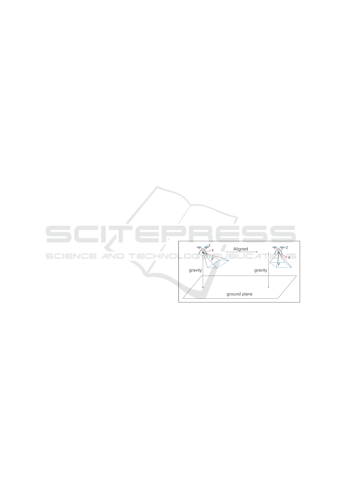
Figure 1: The y-axis of the camera is orthogonal to the
ground plane after being aligned with the gravity direction.
manned aerial vehicles (UAVs), which commonly
feature IMUs capable of measuring the gravitational
vector. Given an uncalibrated smart device, e.g., a
smart phone, we can capture the images and the cor-
responding IMU data which can be used to measure
the gravity direction. As shown in (Kukelova et al.,
2010; Guan et al., 2018), the relationship between the
axes of the camera and the IMU are usually 0°, 90°
or 180°. In this case, the rotation between the camera
and the IMU of smart devices can be known with-
out calibrating the camera and the IMU. We can align
y-axes of the camera with the gravity direction, re-
ducing relative orientation to 1-DoF rotation around
680
Su, Y., Guo, X. and Shen, Y.
Camera Self-Calibration from Two Views with a Common Direction.
DOI: 10.5220/0012438100003660
Paper published under CC license (CC BY-NC-ND 4.0)
In Proceedings of the 19th International Joint Conference on Computer Vision, Imaging and Computer Graphics Theory and Applications (VISIGRAPP 2024) - Volume 3: VISAPP, pages
680-685
ISBN: 978-989-758-679-8; ISSN: 2184-4321
Proceedings Copyright © 2024 by SCITEPRESS – Science and Technology Publications, Lda.

the gravity direction (Fig. 1). A crucial insight is
the general orthogonality between the ground plane
and the gravity direction. This assumption is fulfilled
for many man-made environments, and has been suc-
cessfully used in many computer vision tasks (Dibene
et al., 2023; Li et al., 2023). Leveraging this ground
plane constraint, we propose new homography-based
minimal solutions for camera self-calibration with the
known gravity direction. The proposed framework is
depicted in Fig. 2 The main contributions of this paper
are:
(i) By exploiting the ground plane assumption, we
show that the Euclidean homography matrix has spe-
cial properties which allows us to derive new con-
straints and solve the homography-based camera self-
calibration problem efficiently.
(ii) Based on the new homography-based con-
straints, we derive 2.5-point algorithms for points in
the ground plane to estimate the focal length of the
camera.
(iii) Moreover, we propose a 3.5-point algorithm
to estimate the focal length and principal point coor-
dinates of the camera simultaneously.
2 OUR APPROACH
2.1 Homography-Based Constraints
Suppose two image points m = [u, v,1]
⊤
and m
′
=
[u
′
,v
′
,1]
⊤
are given for a point on a plane in the 3D
space with respect to two camera frames. The Eu-
clidean homography matrix H that transforms one
into the other satisfies
λK
−1
m
′
= HK
−1
m, (1)
where λ is a scaling factor, and K is the camera in-
trinsic matrix. The Euclidean homography matrix H
is related to the rotation matrix R, the translation ma-
trix T, the distance d from the camera frame to the
target plane, and the normal N of the plane according
to
H = R −
1
d
TN
⊤
. (2)
Since the gravity direction can be calculated from the
IMU data, without loss of generality, we can align
the y-axes of the cameras with the gravity direction
(Fig. 1). After alignment, the rotation transformation
matrix of two camera views reduces from 3-DoF to
1-DoF and can be represented as
R
y
=


cosθ 0 sinθ
0 1 0
−sinθ 0 cosθ


. (3)
Applying the rotations to the normalized image
points, then Eq. (1) becomes
λR
⊤
2
K
−1
m
′
= H
y
R
⊤
1
K
−1
m, (4)
with
H
y
= R
y
− tn
⊤
, (5)
where R
1
,R
2
are the rotation matrices of two cameras
for the alignment, t = [t
x
,t
y
,t
z
]
⊤
and n are the transla-
tion and plane parameters after the alignment. Based
on the assumption that the ground planes are orthogo-
nal to the gravity direction, the plane normal n is equal
to [0 1 0]
⊤
when the points lie in a horizontal plane.
Then Eq. (5) can be formulated as
H
y
=


cosθ 0 sinθ
0 1 0
−sinθ 0 cosθ


−


t
x
t
y
t
z


[0 1 0]
=


cosθ −t
x
sinθ
0 1 −t
y
0
−sinθ −t
z
cosθ


.
(6)
Obviously H
y
obeys 4 constraints:
h
4
= 0, h
6
= 0, h
1
− h
9
= 0, h
3
+ h
7
= 0, (7)
where h
i
are the elements of the matrix H
y
. These
constraints allow us to solve minimal solutions for
camera self-calibration more efficiently.
2.2 Unknown Focal Length(2.5-point)
For most modern CCD and CMOS cameras, it is rea-
sonable to assume unit aspect ratio and that the princi-
pal point coincides with the image centerEq.(Hartley
and Li, 2012). In this case, the only unknown intrinsic
camera parameter is the focal length f . We propose a
2.5-point algorithm for estimating f .
In general, Eq. (1) can be written as
λm
′
= Gm, (8)
where G transforms the image points. Given one
point correspondence (m,m
′
), Eq. (8) can also be
written as

0 0 0 -u -v -1 v
′
u v
′
v v
′
u v 1 0 0 0 -u
′
u -u
′
v -u
′

g = 0,
g = [g
1
g
2
g
3
g
4
g
5
g
6
g
7
g
8
g
9
]
⊤
, (9)
where g
1
,g
2
,...,g
9
are the elements of the 2D homog-
raphy matrix G. Each point correspondence gives two
linearly independent constraints. By stacking the con-
straints for κ point correspondences,Eq. (9) leads to a
system of equations of the form
Ag = 0, (10)
Camera Self-Calibration from Two Views with a Common Direction
681

Figure 2: The overall framework of the proposed method.
where A is a 2κ × 9 matrix. Then g and the 2D ho-
mography matrix G can be found as the null space
of A. With 2.5 point correspondences (note that we
still need to use three point correspondences, but only
need one equation from the last correspondence), the
general solution of g in Eq. (10) is a 4-dimensional
null space which can be written as
g = αg
a
+ βg
b
+ γg
c
+ g
d
, (11)
where α, β,γ are the coefficients. Based on Eq. (4) and
Eq. (8), the Euclidean homography matrix H
y
can be
formulated as
H
y
= R
⊤
2
K
−1
GKR
1
. (12)
Let K = diag( f , f ,1), K
−1
= diag(1/ f ,1/ f ,1). Sub-
stituting Eq. (11) into Eq. (12) we can parameterize
H
y
using {α,β,γ, f }. Then substituting this formula-
tion into constraints Eq. (7), we obtain 4 polynomial
equations in 4 unknowns {α,β,γ, f }:
a
i
[1,α,β, γ, f ,α f , β f ,γ f , f
2
,α f
2
,β f
2
,γ f
2
]
⊤
= 0,
(13)
where {a
i
|i = 1, 2,3,4} are coefficients. The system
of equations Eq. (13) can be solved using the Gr
¨
obner
basis method (Cox et al., 2006). For more details
about the Gr
¨
obner basis method and the polynomial
eigenvalue solution we refer the reader to (Kukelova
et al., 2012; Larsson et al., 2017b; Larsson et al.,
2017a; Larsson et al., 2018). There are up to 4 real
solutions. Negative solutions of f can also be aban-
doned.
2.3 Unknown Focal Length and
Principal Point(3.5-point)
However, sometimes the principal point may not co-
incide with the image center. In this case, the un-
known camera intrinsic parameters are the unknown
focal length f and the principal point (u
0
,v
0
). Let
K =


f 0 u
0
0 f v
0
0 0 1


,K
−1
=


1/ f 0 −u
0
/ f
0 1/ f −v
0
/ f
0 0 1


.
(14)
We derive a 3.5-point algorithm to estimate the cam-
era intrinsic parameters. With 3.5 point correspon-
dences, the general solution of g in Eq. (10) is a 2-
dimensional null space which can be written as
g = αg
a
+ g
b
. (15)
Substituting Eq. (14) and Eq. (15) into Eq. (12) we
can parameterize H
y
using {α, f ,u
0
,v
0
}. Then sub-
stituting this formulation into constraints Eq. (7),
we obtain 4 polynomial equations in 4 unknowns
{α, f , u
0
,v
0
}:
b
i
[1,α, f ,u
0
,v
0
,α f , αu
0
,αv
0
, f u
o
, f v
0
,u
0
v
0
,·· ·
α f u
0
,α f v
0
,αu
0
v
0
, f
2
,u
2
0
,v
2
0
,α f
2
,αu
2
0
,αv
2
0
]
⊤
= 0,
(16)
where {b
i
|i = 1,2,3,4} are coefficients. Here we rec-
ommend using an automatic generator to solve the
system of polynomial equations, e.g. , (Larsson et al.,
2017a). We obtain a Gauss-Jordan elimination tem-
plate of size 79 × 91, and there are up to 12 real solu-
tions.
3 EXPERIMENTS
We choose the following setup to generate the syn-
thetic data for the self-calibration evaluation. It con-
tains two image sequences. The simulated cameras
of both sequences have the same parameters: the fo-
cal length f
g
of the camera is set to 3442 pixels, and
the coordinates of the principal point (u
g
,v
g
) is set
to (2016,1512). The image resolution of the first
sequence is 4032 × 3024, i.e., the principal point of
the camera coincides with the image center. The im-
age resolution of the second sequence is 3225 × 2419
which indicates that the principal point does not lo-
cate at the center of the image. 100 3D points are
distributed on the ground plane which is orthogonal
to the image plane of the first view. Each 3D point
is observed by two camera views to generate an im-
age pair. This is similar to (Fraundorfer et al., 2010;
Saurer et al., 2017; Ding et al., 2022). We generate
1,000 pairs of images for each sequence to evaluate
the performance. The relative focal length error is de-
VISAPP 2024 - 19th International Conference on Computer Vision Theory and Applications
682

(a) the first sequence (b) the second sequence
Figure 3: Histograms of the relative focal length error E
f
distribution for 10,000 runs with the first and the second
image sequences, respectively.
fined as
E
f
= | f
e
− f
g
|/ f
g
, (17)
where f
e
denotes the estimated focal length and f
g
is
the ground truth. The principal point error is formu-
lated as
E
uv
=
q
(
|
(u
e
− u
g
)
|
/u
g
) ∗ (
|
(v
e
− v
g
)
|
/v
g
), (18)
where (u
e
,v
e
) denotes the estimated coordinates of
the principal point and (u
g
,v
g
) is the true one.
3.1 Numerical Precision
Figure 3 shows the histograms of the relative focal
length error E
f
of the proposed algorithms for 10,000
runs with the first and the second image sequences,
respectively. ’2.5pt’ denoteS the 2.5-point algorithms
using the Gr
¨
obner basis solution. ’3.5pt’ denotes the
3.5-point algorithms using the Gauss-Jordan elimina-
tion template of size 79 ×91. The error distribution of
Fig. 3(a) shows that the 2.5-point algorithm performs
as expected for the focal length estimation when the
principal point of the camera coincides with the im-
age center. The stability of 3.5-point algorithm is not
as good as the 2.5-point case, but it does not contain
large errors and is sufficient for real applications. As
shown in Fig. 3(b), the 3.5-point algorithm is more
reliable than the 2.5-point algorithm when the princi-
pal point of the camera does not locate at the center
of the image. Figure 4 shows the principal point error
E
uv
of the 3.5-point algorithm for 10,000 runs with the
first and the second image sequences, respectively. As
shown, our method is efficient and robust in estimat-
ing the principal point of the camera on both of the
image sequences.
3.2 Stability of the Solutions Compared
to Other Methods
In this section we compare the proposed methods with
the state of the arts. ’6pt’ denotes the two-view 6-
point algorithm proposed in (Kukelova et al., 2017).
(a) the first sequence (b) the second sequence
Figure 4: Histograms of the principal point error E
uv
distri-
bution for 10,000 runs with the first and the second image
sequences, respectively.
’4pt’ denotes the 4-point homography based algo-
rithm proposed in (Ding et al., 2022). Because we
still need to sample 3 and 4 points in practice, we use
SVD to compute the null space with 3 and 4 points,
respectively. These algorithms are evaluated under in-
creased level of image noise (point location) from 0 to
1 pixel. In addition, the gravity direction measured by
the accelerometers is not perfect in real environment.
Thus we also simulate the noisy case with increased
roll, pitch noise (gravity direction) and constant im-
age noise of 0.5 pixel standard deviation. The max
standard deviation of the (roll, pitch) noise is set to
0.5
◦
, because smart phone IMUs typically have noise
of less than 0.5
◦
(Sweeney et al., 2014). Note that for
our algorithms we use the noisy roll, pitch angles to
compute the full rotation.
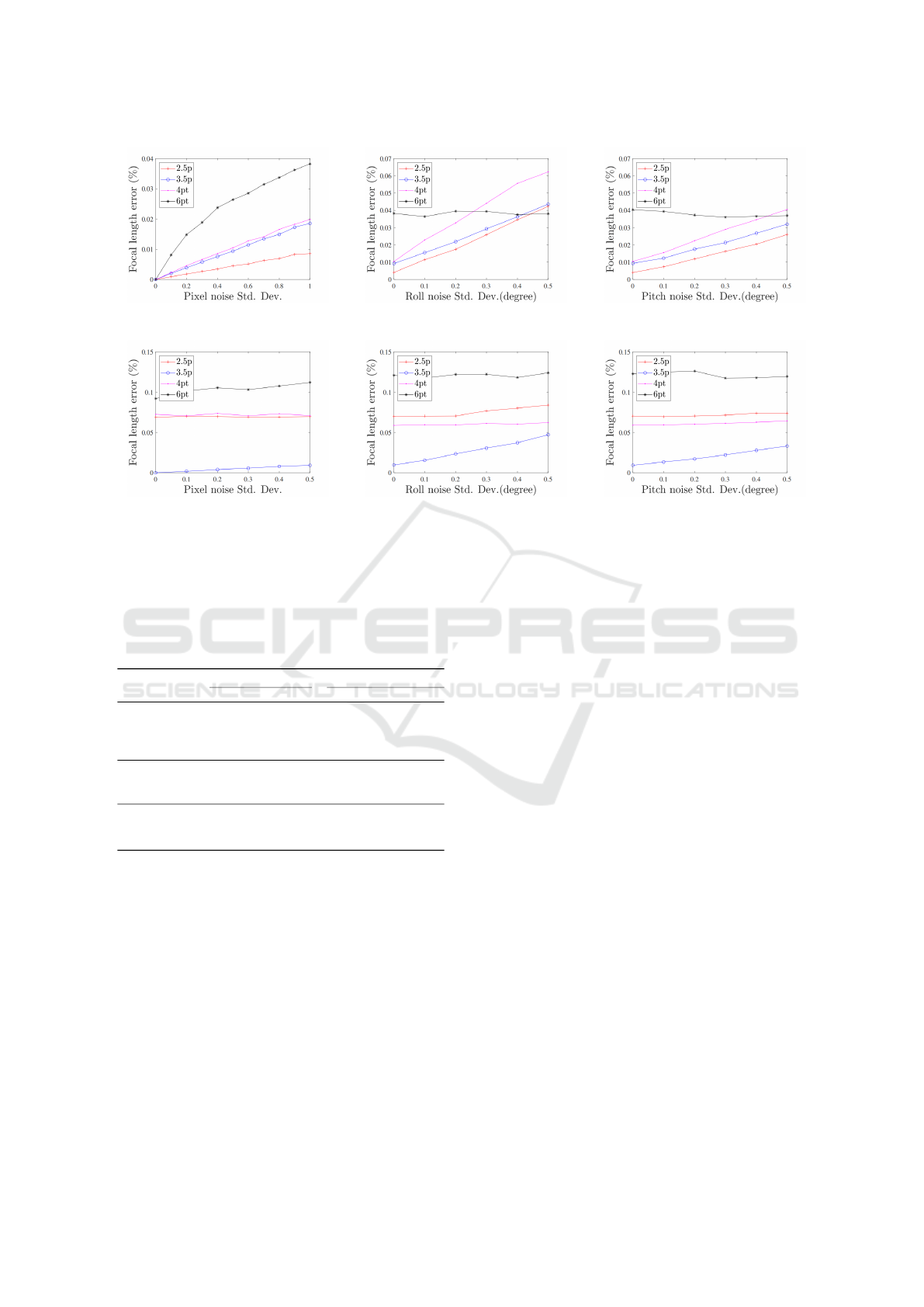
Figure 5 shows the median focal length error of
the first image sequence (the first row) and the sec-
ond image sequence (the second row) with increased
image noise (the left column), roll noise (the mid-
dle column) and pitch noise (the right column), re-
spectively. As expected, the proposed 2.5-point al-
gorithm performs better than the other ones under
perfect IMUs data and the 3.5-point algorithm can
also achieve promising results for estimating the fo-
cal length of camera when the principal point of the
camera locates at the center of the image (as shown in
Fig. 5(a)). Figure 5(b) shows that the proposed 3.5-
point algorithm is more accurate than the other three
methods when the principal point of the camera does
not coincide with the image center. The 6pt algorithm
is not influenced by the roll and pitch noise because it
does not need IMUs data. Overall, we can see that the
proposed 2.5- and 3.5-point algorithms are slightly
better than the other methods on focal length estima-
tion when the principal point of the camera does and
does not coincide with the image center, respectively.
Camera Self-Calibration from Two Views with a Common Direction
683

(a) the first image sequence
(b) the second image sequence
Figure 5: Boxplot of relative focal length error. The results of the first column are with the increased image noise from 0 to 1
pixel. The results of the second column are with the increased roll noise from 0 to 0.5
◦
and the constant image noise of 0.5
pixel. The results of the last column are with the increased pitch noise from 0 to 0.5
◦
and the constant image noise of 0.5
pixel.
Table 1: The principal point error E
uv
of the 3.5-point al-
gorithm with the synthetic data for 10,000 runs under both
image sequences.
the first sequence the second sequence
mean median mean median
Image
noise
0
1.153
e-09
1.8685
e-13
1.2959
e-09
1.8688
e-13
0.5 0.0396 0.012 0.0405 0.0119
1.0 0.0704 0.0241 0.0692 0.0237
Roll
noise
0.1 0.0496 0.0193 0.0462 0.0187
0.3 0.1060 0.0457 0.1134 0.0534
0.5 0.1503 0.0666 0.1537 0.0782
Pitch
noise
0.1 0.0471 0.0192 0.0460 0.0184
0.3 0.0705 0.0305 0.0687 0.0295
0.5 0.0919 0.0438 0.0877 0.0433
3.3 Evaluation of the Principal Point
To our best knowledge, no homography-based two
view method has been performed to estimate the prin-
cipal point. So we only give the statistical results of
our method without the comparisons to other meth-
ods. Table 1 gives the principal point error E
uv
of the
3.5-point algorithm with the synthetic data for 10,000
runs under both image sequences. Similarly, we eval-
uate the 3.5-point algorithm under increased level of
image noise and roll, pitch noise. The third and the
fourth column show the results of the first image se-
quence (the principal of the camera coincides with the
image center). The fifth and the sixth column give the
results of the second image sequence (the principal
point does not locate at the image center). The third to
the fifth rows show the principal point error E
uv
with
the increased image noise from 0 to 1 pixel. The sixth
to the eighth rows show the results with the increased
roll noise from 0 to 0.5 degree and the constant im-
age noise of 0.5 pixel standard deviation. The last
three rows shows the results with the increased pitch
noise from 0 to 0.5 degree and the constant image
noise of 0.5 pixel. As shown, the proposed method
can achieve efficient results for the principal point es-
timation under different noise cases and sequences.
In general, based on the simulation experiments
we find that the proposed 2.5- and 3.5-point algo-
rithms are comparable to the existing methods for the
focal length and the principal point estimation under
different noise cases. To the best of our knowledge,
good IMUs today can have noise levels of around 0.06
degrees in the computed angles (Fraundorfer et al.,
2010). In this case, our algorithms are practical and
can be used as alternative algorithms on camera self-
calibration pipelines for smart phones and tablets.
VISAPP 2024 - 19th International Conference on Computer Vision Theory and Applications
684

4 CONCLUSION
This paper proposes a self-calibration method for
estimating camera focal length and principal point
based on the orthogonality assumption and homog-
raphy constraints. Leveraging IMU data and the or-
thogonality assumption, new homography constraints
are derived in this paper. The 2.5-point and 3.5-point
methods for estimating camera focal length and prin-
cipal point are presented. Thanks to the simplified
constraints, the algorithm in this paper not only ex-
hibits superior performance compared to alternative
approaches but also ensures high efficiency. We be-
lieve that the method proposed in this paper can serve
as an alternative algorithm for camera self-calibration
in intelligent vehicle applications, further enhancing
the performance of intelligent vehicle systems.
ACKNOWLEDGEMENTS
The authors would like to thank the editor and
the anonymous reviewers for their critical and con-
structive comments and suggestions. This work is
supported by Suqian science and technology plan
project under No. K202233, K202229, K202231,
H202117 and Suqian Natural Science Foundation
(No. M202305).
REFERENCES
Cox, D. A., Little, J., and O’shea, D. (2006). Using al-
gebraic geometry, volume 185. Springer Science &
Business Media.
Dibene, J. C., Min, Z., and Dunn, E. (2023). General planar
motion from a pair of 3d correspondences. In Pro-
ceedings of the IEEE/CVF International Conference
on Computer Vision, pages 8060–8070.
Ding, Y., Barath, D., Yang, J., and Kukelova, Z. (2022).
Relative pose from a calibrated and an uncalibrated
smartphone image. In Proceedings of the IEEE/CVF
Conference on Computer Vision and Pattern Recogni-
tion, pages 12766–12775.
Fitzgibbon, A. (2001). Simultaneous linear estimation of
multiple view geometry and lens distortion. In Pro-
ceedings of the 2001 IEEE Computer Society Con-
ference on Computer Vision and Pattern Recognition.
CVPR 2001.
Fraundorfer, F., Tanskanen, P., and Pollefeys, M. (2010). A
minimal case solution to the calibrated relative pose
problem for the case of two known orientation an-
gles. In The European Conference on Computer Vi-
sion (ECCV).
Guan, B., Yu, Q., and Fraundorfer, F. (2018). Minimal solu-
tions for the rotational alignment of imu-camera sys-
tems using homography constraints. Computer vision
and image understanding.
Hartley, R. and Li, H. (2012). An efficient hidden variable
approach to minimal-case camera motion estimation.
IEEE transactions on pattern analysis and machine
intelligence.
Kukelova, Z., Bujnak, M., and Pajdla, T. (2010). Closed-
form solutions to minimal absolute pose problems
with known vertical direction. In Asian Conference
on Computer Vision.
Kukelova, Z., Bujnak, M., and Pajdla, T. (2012). Poly-
nomial eigenvalue solutions to minimal problems in
computer vision. IEEE Transactions on Pattern Anal-
ysis and Machine Intelligence.
Kukelova, Z., Heller, J., Bujnak, M., and Pajdla, T. (2015).
Radial distortion homography. In The IEEE Con-
ference on Computer Vision and Pattern Recognition
(CVPR).
Kukelova, Z., Kileel, J., Sturmfels, B., and Pajdla, T.
(2017). A clever elimination strategy for efficient min-
imal solvers. In The IEEE Conference on Computer
Vision and Pattern Recognition (CVPR).
Larsson, V.,
˚
Astr
¨
om, K., and Oskarsson, M. (2017a). Ef-
ficient solvers for minimal problems by syzygy-based
reduction. In The IEEE Conference on Computer Vi-
sion and Pattern Recognition (CVPR).
Larsson, V., Astrom, K., and Oskarsson, M. (2017b). Poly-
nomial solvers for saturated ideals. In The IEEE In-
ternational Conference on Computer Vision (ICCV).
Larsson, V., Oskarsson, M.,
˚
Astr
¨
om, K., Wallis, A.,
Kukelova, Z., and Pajdla, T. (2018). Beyond gr
¨
obner
bases: Basis selection for minimal solvers. In The
IEEE Conference on Computer Vision and Pattern
Recognition (CVPR).
Li, H., Zhao, J., Bazin, J.-C., Kim, P., Joo, K., Zhao, Z.,
and Liu, Y.-H. (2023). Hong kong world: Leveraging
structural regularity for line-based slam. IEEE Trans-
actions on Pattern Analysis and Machine Intelligence.
Nist
´
er, D. (2004). An efficient solution to the five-point
relative pose problem. IEEE transactions on pattern
analysis and machine intelligence.
Saurer, O., Vasseur, P., Boutteau, R., Demonceaux, C.,
Pollefeys, M., and Fraundorfer, F. (2017). Homog-
raphy based egomotion estimation with a common di-
rection. IEEE transactions on pattern analysis and
machine intelligence.
Sweeney, C., Flynn, J., and Turk, M. (2014). Solving
for relative pose with a partially known rotation is a
quadratic eigenvalue problem. 3DV.
Zhang, Z. (2000). A flexible new technique for camera cal-
ibration. IEEE Transactions on pattern analysis and
machine intelligence, 22.
Camera Self-Calibration from Two Views with a Common Direction
685