BornFS: Feature Selection with Balanced Relevance and Nuisance and

Its Application to Very Large Datasets

Kilho Shin

1 a

, Chris Liu

, Katsuyuki Maeda

and Hiroaki Ohshima

3 b

Computer Centre, Gakushuin University, Mejiro, Tokyo, Japan

Deloitte Tohmatsu Cyber LLC., Marunouchi, Tokyo, Japan

Graduate School of Information Science, University of Hyogo, Kobe, Hyogo, Japan

Keywords:

Feature Selection, Categorical Data.

Abstract:

In feature selection, we grapple with two primary challenges: devising effective evaluative indices for selected

feature subsets and crafting scalable algorithms rooted in these indices. Our study addresses both. Beyond

assessing the size and class relevance of selected features, we introduce a groundbreaking index, nuisance.

It captures class-uncorrelated information, which can muddy subsequent processes. Our experiments conﬁrm

that a harmonious balance between class relevance and nuisance augments classiﬁcation accuracy. To this

end, we present the Balance-Optimized Relevance and Nuisance Feature Selection (BornFS) algorithm. It not

only exhibits scalability to handle large datasets but also outperforms traditional methods by achieving better

balance among the introduced indices. Notably, when applied to a dataset of 800,000 Windows executables,

using LCC as a preprocessing ﬁlter, BornFS slashes the feature count from 10 million to under 200, maintain-

ing a high accuracy in malware detection. Our ﬁndings shine a light on feature selection’s complexities and

pave the way forward.

1 INTRODUCTION

Feature selection is pivotal in machine learning and

gains prominence with increasing data. With big

data introducing myriad features, efﬁcient feature se-

lection is paramount. For example, in bioinformat-

ics, datasets may feature thousands of genes, making

identifying disorder-linked genes a feature selection

challenge. As machine learning progresses, reﬁned

feature selection becomes critical.

While dimensionality reduction is often equated

with feature selection, they are distinct concepts. Di-

mensionality reduction is generally applied to contin-

uous features, crafting new dimensions that encap-

sulate the essence of the original dataset. In con-

trast, feature selection, which has undergone exten-

sive study particularly for categorical features, in-

volves choosing from the existing features.

Deep neural networks are also gaining attention

for their ability to effectively extract features from

data. However, these extracted features are typically

not human-interpretable, contrasting with feature se-

https://orcid.org/0000-0002-0425-8485

https://orcid.org/0000-0002-9492-2246

lection, which directly identiﬁes important features.

This paper delves into categorical feature selec-

tion, crucial for tasks like pinpointing disease-causing

genes. Categorical feature selection has seen thor-

ough exploration in literature, as demonstrated by

(Almuallim and Dietterich, 1994; Hall, 2000; Yu and

Liu, 2003; Peng et al., 2005; Zhao and Liu, 2007;

Shin et al., 2015).

This paper addresses two primary challenges in

modern categorical feature selection:

1. Feature Evaluation Indices: We’ve introduced ro-

bust indices for assessing feature subset quality.

Apart from the conventional high class relevance

and few feature count indices, a novel low nui-

sance metric is presented. This quantiﬁes non-

class-related information in the feature subset.

2. Algorithmic Innovation with Scalability: We

present BORNFS, an algorithm tailored to bal-

ance the three indices and adeptly process large

datasets.

This paper begins with an overview of categori-

cal feature selection algorithms, introducing the new

nuisance index and an aggregate index for class rel-

evance balance. We conduct two experiments: ﬁrst,

1100

Shin, K., Liu, C., Maeda, K. and Ohshima, H.

BornFS: Feature Selection with Balanced Relevance and Nuisance and Its Application to Very Large Datasets.

DOI: 10.5220/0012436000003636

Paper published under CC license (CC BY-NC-ND 4.0)

In Proceedings of the 16th International Conference on Agents and Artiﬁcial Intelligence (ICAART 2024) - Volume 3, pages 1100-1107

ISBN: 978-989-758-680-4; ISSN: 2184-433X

analyzing the balance in compact datasets and then in

16 larger benchmark datasets. Results show a corre-

lation between balance and predictive accuracy, lead-

ing to our new mechanism, BORNFS. We compare its

performance with mRMR and LCC, concluding with

an experiment using BORNFS on a dataset with over

10 million features and 800,000 instances.

2 MATHEMATICAL NOTATIONS

A dataset D is represented as a matrix with n

rows

corresponding to instances and n

+ 1 columns cor-

responding to features. The rightmost column rep-

resents the class labels of the instances, while the

other columns are denoted as F

,...,F

. We focus

on datasets where all features are categorical, thus,

the value set R(F) for a feature F, including F

or the

class featureC, is ﬁnite.

In this context, the dataset deﬁnes a probability

measure over the sample space Ω

= R(F

) × · · · ×

R(F

) × R(C). The empirical probability for a vec-

tor v

v ∈ Ω

is given by P

,...,F

,C = v

v] =

n(v

where n(v

v) denotes the number of occurrences of v

Here, both features and the class feature are consid-

ered random variables, allowing the application of

probability-based metrics such as entropy and mutual

information.

3 RELATED WORK

3.1 Relevance, Redundancy, Interaction

Many studies posit the ultimate goal of feature selec-

tion as the identiﬁcation of the smallest subset of fea-

tures that exhibits the highest class relevance. This

class relevance pertains to the collective correlation

of a feature subset F with class labels. Various mea-

sures, such as mutual information I(F ;C), are used to

quantify this relevance.

To achieve this goal, several algorithms in the lit-

erature, including CFS (Hall, 2000), RELIEF-F (Kira

and Rendell, 1992), and mRMR (Zhao et al., 2019),

capitalize on the concept of internal redundancy. This

concept refers to the shared information among fea-

tures, where reducing redundancy helps decrease the

feature count. For instance, when considering the in-

clusion of a feature F in a feature set F , these al-

gorithms assess the balance between redundancy gain

and relevance gain. These gains can be estimated as

I(F ; F) and I(F ,F;C) − I(F ;C), respectively.

In evaluating I(F ;F), the approximation

I(F ; F) ≈

∑

∈F

I(F

;F) is common, enhancing

time efﬁciency but potentially missing critical feature

interactions. Advanced methods like INTERACT by

(Zhao and Liu, 2007) and its successors like LCC

(Shin et al., 2011; Shin et al., 2017) have reﬁned

feature selection, considering these interactions for

improved relevance and feature count.

3.2 Advances in Time Efﬁciency

To select k features that maximize class relevance, ex-

haustive search typically requires O(n

) time. Algo-

rithms like mRMR, CFS, and RELIEF-F improve this

to O(k

), effectively balancing relevance and re-

dundancy. Even more efﬁcient, LCC further reduces

the time complexity to O(n

logn

), despite incor-

porating feature interaction into the selection process.

In practical terms, LCC is currently the only ad-

vanced feature selection algorithm known to scale ef-

fectively to big data, as evidenced by its performance

on the DOROTHEA dataset of 100,000 features and

800 instances, where it operates signiﬁcantly faster

than mRMR in Weka, completing the task in under

300 milliseconds versus more than 3,500 seconds.

3.3 The Algorithm of LCC

To achieve both theoretical and practical time efﬁ-

ciency while grounding on the indices introduced, we

develop BORNFS, building upon the algorithmic efﬁ-

ciency and foundation established by LCC.

Input: A dataset D described by F

∪ {C}; and a

threshold t ∈ [0,1].

Output: A minimal feature subset F ⊆ F

with

1 − Br(F ;C) ≥ t (1 − Br(F

;C)).

1 Number the features of F

so that F

,... , F

are in

an increasing order of SU(F

;C).;

2 F =

0 and i = 1.;

3 while i ≤ n

4 Let j = min{ j ∈ [i, n

] | 1 − Br(F ∪ F

[ j +

1,n

];C) < t (1 − Br(F

;C))}.;

5 F = F

∪ { j} and i = j + 1. ;

6 end

7 return F .

Algorithm 1: LCC.

Algorithm 1 outlines the LCC algorithm. To deter-

mine the class relevance, it utilizes the complement of

the Bayesian risk:

1 − Br(F ;C) =

∑

v∈R(F )

max

c∈R(C)

Pr[C = c | F = v

v].

Exploiting the relevance measure’s monotonicity, that

is, 1 − Br(F ;C) ≥ 1 − Br(G;C) for F ⊃ G, LCC em-

ploys binary search to implements Line 4.

BornFS: Feature Selection with Balanced Relevance and Nuisance and Its Application to Very Large Datasets

1101

The sorting step (Line 1) utilizes the normalized

mutual information metric SU(F;C) =

2·I(F;C)

H(F)+H(C)

. In-

troduced empirically to boost classiﬁcation accuracy,

as suggested in (Zhao and Liu, 2007), this sorting

method has proven effective. Features ranked earlier

by this metric are more likely to be eliminated in Line

4, thus optimizing the selection process and enhanc-

ing the overall accuracy of the algorithm.

4 THE THIRD INDEX –

NUISANCE

4.1 Deﬁnition

In addition to established indices such as class rele-

vance and feature count, we introduce an additional

criterion: nuisance.

The term nuisance denotes the portion of informa-

tion within a feature subset unrelated to class labels.

As the primary goal of feature selection is to enhance

the representational ability of features for class labels,

any data not contributing to this objective is consid-

ered redundant, potentially leading to inaccurate pre-

dictions. Nuisance misleads classiﬁers by introducing

irrelevant information. It can be quantiﬁed in various

ways, including:

• Conditional Entropy: H(F | C) = H(F )−I(F ;C)

• Inverted Bayesian Risk Br(C;F ):

• Ratio:

H(F )

I(F ;C)

4.2 Balancing Relevance and Nuisance

To effectively balance class relevance and nuisance,

a robust measure is necessary. Our study utilizes the

harmonic mean of

I(F ;C)

I(F

;C)

for normalized class rele-

vance and

I(F ;C)

H(F )

as the reciprocal of nuisance’s ratio

representation as the primary metric. This metric is

particularly chosen for its sensitivity to both relevance

and nuisance, ensuring that it approaches zero in cases

of low relevance or high nuisance. It is formulated as:

(F ;C) =

2 · I(F ;C)

I(F

;C) + H(F )

. (1)

However, our methodology is ﬂexible and not lim-

ited to this speciﬁc metric alone. Alternative methods

to quantify nuisance and various functions to evaluate

the balance between relevance and nuisance are also

viable and can be integrated into our approach, allow-

ing for adaptability and optimization according to dif-

ferent dataset characteristics and analytical needs.

The selected metric, µ

(F ;C), has the following

properties:

1. µ

(F ;C) = 0 is equivalent to I(F ;C) = 0;

2. µ

(F ;C) = 1 implies I(F ;C) = I(F

;C) =

H(F );

3. When I(F

;C) = H(C), µ

(F ;C) coincides with

SU(F ;C).

5 EFFICACY VALIDATION OF

THE PROPOSED INDICES

We evaluated three indices, particularly the balance

index µ

, across two experiments linking µ

scores to

predictive accuracy. The ﬁrst explored all feature sub-

sets in compact datasets, while the second assessed

sampled subsets in larger benchmark datasets.

5.1 Data Preparation

Before experiments, datasets underwent discretiza-

tion into ten equal parts and binarization, resulting in

binary features, except for class variables, using one-

hot encoding.

5.2 Evaluation of Predictive Accuracy

To evaluate the classiﬁcation power of each feature

subset, we perform ﬁve-fold cross-validation on the

narrowed dataset using LightGBM (LGBM) and Mul-

tiple Layer Perceptron (MLP) classiﬁers.

5.2.1 Experiment 1: Exhaustive Investigation

with Small Datasets

For this experiment, we work with the three MONKS

datasets. While each of these datasets contains the

same 432 instances and is described by six features,

their annotations differ, as outlined in (Blake and

Merz, 1998). After binarization, these datasets are

represented by 17 binary features alongside a class

variable.

For each binarized MONKS dataset, we examine

all 2

− 1 non-empty feature subsets. These subsets

are evaluated based on their µ

scores and AUC-ROC

values using the LGBM and MLP classiﬁers.

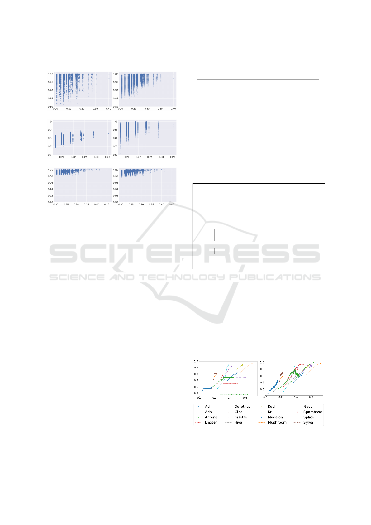
Figure 1 illustrates the correlation between the

(F ;C) scores (represented on the x-axis) and the

AUC-ROC scores (on the y-axis) for feature subsets.

Given that 2

− 1 represents a considerably large

number, the plot is limited to those F with the highest

I(F ;C). The ﬁgure demonstrates that as the µ

(F ;C)

values increase, the AUC-ROC scores increasingly

ICAART 2024 - 16th International Conference on Agents and Artiﬁcial Intelligence

1102

LGBM MLP

MONKS 1 (I(F ;C) = 1.0)

MONKS 2 (I(F ;C) ≥ 0.91)

MONKS 3 (I(F ;C) ≥ 0.99)

Figure 1: Relation between µ

(x axis) and AUC-ROC (y

axis) for the MONKS datasets.

converge within narrower and elevated ranges. This

observation implies a substantial probability of attain-

ing feature subsets with enhanced predictive perfor-

mance by using high µ

(F ;C) scores as a criterion

for selection.

5.2.2 Experiment 2: Investigation with Larger

Datasets

In our second experiment, we examine 15 larger

datasets listed in Table 1. Ten were part of fea-

ture selection challenges at NIPS 2003 (NIPS, 2003)

and WCCI 2006 (WCCI, 2006). One comes from

the KDD 1999 network intrusion detection chal-

lenge (KDD, 1999), while others are from the UCI

repository (Blake and Merz, 1998).

Given the larger number of features in these

datasets, an exhaustive evaluation similar to our ﬁrst

experiment isn’t viable. To pinpoint succinct feature

subsets, F , with prominent µ

scores, we turn to a

hill-climbing sampling method, as outlined in Algo-

rithm 2. This approach yields subsets F

⊂ ··· ⊂ F

for each dataset, where the size of subset F

is i and it

meets the condition µ

;C) < µ

i+1

;C).

Figure 2 showcases the relationship between

the AUC-ROC scores (on the y-axis) and the µ

scores (plotted on the x-axis) for each feature sub-

set F

produced by Algorithm 2. Excluding two

exceptions-—DEXTER with LGBM and DOROTHEA

with MLP—-there is a discernible positive correlation

between the predictive performance of the classiﬁers

Table 1: Attributes of datasets.

Dataset #F #BF #I Ref.

AD 1,559 3,137 3,279 (Blake and Merz, 1998)

ADA 49 134 4,147 (WCCI, 2006)

ARCENE 10,001 83,950 100 (NIPS, 2003)

DEXTER 20,001 35,924 300 (NIPS, 2003)

DOROTHEA 100,001 100,001 800 (NIPS, 2003)

GINA 971 9,683 3,153 (WCCI, 2006)

GISETTE 5,001 39,809 6,000 (NIPS, 2003)

HIVA 1,618 3,235 3,845 (WCCI, 2006)

KDD 42 346 25,192 (KDD, 1999)

KR 37 74 3,196 (Blake and Merz, 1998)

MADELON 501 4,972 2,000 (NIPS, 2003)

MUSHROOM 23 114 8,124 (Blake and Merz, 1998)

NOVA 16,970 29,368 1,754 (WCCI, 2006)

SPAMBASE 58 134 4,601 (Blake and Merz, 1998)

SYLVA 217 746 13,086 (WCCI, 2006)

Input: A dataset described by a feature set F

and

Output: Feature subsets F

⊂ ·· · ⊂ F

with |F

| = i.

1 Let n = 0 and F

2 while true do

3 Let F ∈ argmax µ

,F;C);

4 if µ

,F;C) > µ

;C) then

5 Let n = n + 1;

6 F

= F

n−1

∪ {F};

7 else

8 return F

,. . . , F

9 end

10 end

Algorithm 2: A hill-climbing sampling.

and the µ

scores of their corresponding feature sub-

sets. Especially with MLP, this positive correlation is

strongly evident across all the datasets.

5.3 Conclusions from the Experiments

Both experiments afﬁrm the effectiveness of nuisance

in feature selection and the metric µ

for capturing

feature set nature.

LGBM

MLP

Figure 2: Relation between µ

(x axis) and AUC-ROC (y

axis) for larger datasets.

BornFS: Feature Selection with Balanced Relevance and Nuisance and Its Application to Very Large Datasets

1103

6 A NEW ALGORITHM – BORNFS

We introduce the ﬁrst categorical feature selection al-

gorithm assessing nuisance, class relevance, and fea-

ture count, named Balance-Optimized Relevance and

Nuisance Feature Selection (BORNFS). It’s highly

time-efﬁcient, scalable to large datasets.

6.1 Design Policies of BORNFS

Class relevance ought to be given the highest priority

among the three indices. This prioritization ensures

that the most signiﬁcant factor inﬂuencing the algo-

rithm’s effectiveness is appropriately emphasized.

Speciﬁcally, I(F ;C) gauges the information cru-

cial for accurate understanding and effective learn-

ing. A feature set’s signiﬁcance is compromised if

its class relevance is low, regardless of its size or nui-

sance level.

To manage class relevance, we introduce t

abundance and t

t-minimality, guided by a threshold

t ∈ (0, 1]. Our algorithm seeks to yield feature sub-

sets adhering to these criteria.

Deﬁnition 1. Given a dataset D described by a fea-

ture set F

and a threshold t ∈ (0, 1], the criteria

of t-abundance and t-minimality for a feature subset

F ⊆ F

are deﬁned as:

1. t

t-abundance:

I(F ;C)

I(F

;C)

≥ t ;

2. t

t-minimality:

I(G;C)

I(F

;C)

< t for any G $ F .

The fulﬁllment of t-abundance ensures that the

feature subset possesses adequate relevance, while t-

minimality reduces the feature count. Therefore, our

revised objective is to develop a fast algorithm that

selects feature subsets which are both t-abundant and

t-minimal, and that also exhibit low nuisance.

6.2 The Key Idea

In developing BORNFS, we adapted the LCC frame-

work for its signiﬁcant speed and ability to scale to

very large datasets. The key feature contributing to

the efﬁciency of LCC is its iterative binary search rou-

tine, which selects a single feature per iteration. For

BORNFS, we customized it to be guided by the t-

abundance principle.

Moreover, before executing each binary search,

BORNFS arranges the features within the search

range based on an estimation of potential gains in

relevance and nuisance. To optimize the balance,

BORNFS leverages the property of the LCC search

framework where features positioned later are more

likely to be selected.

When using F to denote the set of features se-

lected prior to the next search, we express the poten-

tial gain in relevance as ∆

(F; F ) and the potential

gain in nuisance as ∆

(F;F ) as follows:

∆

(F;F ) = I(F , F;C) − I(F ;C); (2)

∆

(F;F ) = H(F) − I(F; F ,C). (3)

The algorithm is designed to swiftly update these val-

ues following the addition of a new feature to F .

While the introduction of this sorting procedure

causes computational overhead, it does not affect the

overall asymptotic time complexity, as detailed in

(Section 7.1).

6.3 Algorithm Description

Algorithm 3 describes BORNFS.

6.3.1 Fundamental Structure

The algorithm iteratively selects features, choosing

one from a search range during each cycle. Let’s de-

ﬁne:

• F as the set of previously chosen features;

• The current search range as F

,...,F

When the algorithm calculates r

I(F ,F

i+1

,...,F

;C)

I(F

;C)

for i ∈ [s, n

], if r

≥ t, it considers features F

,...,F

as insigniﬁcant according to t-abundance.

As the ratio decreases with increasing i, a binary

search efﬁciently ﬁnd the value:

∗

= min



i ∈ [s, n

]



I(F , F

i+1

,...,F

;C)

I(F

;C)

< t



Upon ﬁnding s

∗

, BORNFS includes F

∗

in F and

shifts the search range to F

∗

,...,n

6.3.2 Sorting of Features in a Search Range

In the iterative process of identifying s

∗

, features posi-

tioned earlier in the search range are more likely to be

omitted, as indicated by previous studies (Zhao and

Liu, 2007; Shin et al., 2017). Leveraging this insight,

BORNFS sorts features based on their potential im-

pact on the balance between relevance and nuisance.

To assess the impact, BORNFS employs one of the

following:

Ratio: Γ

(F;F ) =

∆

(F;F )

∆

(F; F )

;

Harmonic mean: Γ

(F;F ) =

2(I(F ;C) + ∆

(F; F ))

I(F

;C) + H(F )+ ∆

(F; F ) + ∆

(F; F )

ICAART 2024 - 16th International Conference on Agents and Artiﬁcial Intelligence

1104

Furthermore, the execution speed of BORNFS is

impacted by the frequent sorting process using either

or Γ

. To mitigate this, BORNFS introduces a

hop parameter, denoted as h, which dictates that sort-

ing occurs every h iterations. Essentially, LCC can be

considered a variant of BORNFS with an inﬁnite hop

value (h = ∞).

Input: A dataset described by F

∪ {C}; t ∈ (0, 1];

one of Γ

and Γ

; and a hop h ∈ N.

Output: A t-abundant and t-minimal F ⊆ F

1 Let F =

0. Let s = 1 and c = 0. while s ≤ n

2 if c mod h ≡ 0 then

3 Renumber F

,. . . , F

in an increasing order

of Γ(F; F );

4 else

5 end

6 if ∃s

∗

= min

i ∈ [s, n

]



I(F ,F

i+1

,...,F

;C)

I(F

;C)

< t

then

7 Let F = F ∪ {F

∗

}.;

8 Let s = s

∗

+ 1. ;

9 else

10 return F .

11 end

12 Increment c by one.;

13 end

14 return F .

Algorithm 3: Born Feature Selection (BORNFS).

7 COMPARING BORNFS WITH

LCC AND mRMR

In this section, we juxtapose LCC, mRMR, and

BORNFS concerning asymptotic computational com-

plexity, real-time efﬁciency, and the quality of their

outputs.

Algorithm Source

BORNFS Java executable codes available at (Shin

and Maeda, 2023)

mRMR C++ codes crafted by its creators,

sourced from (Peng, 2007).

LCC Java executable codes by its creators,

sourced from (Shin et al., 2015)

7.1 Asymptotic Time Complexity

The average time complexity of mRMR is O(k

where k denotes the number of features to select, and

that of LCC is O(n

logn

). In this section, we

demonstrate that the time complexity of BORNFS is

also O(n

logn

To analyze, for the ith iteration of selecting a fea-

ture, F

i−1

denotes the previously selected feature set,

and `

is a random variable representing the size of

the search range in the current iteration. For ease of

analysis, we consider `

as a continuous variable span-

ning the range [0,n

]. When f

(x) is the probabil-

ity density function of `

, f

(x|`

i−1

= t) =

holds for

x ∈ (n

−t, n

]. Thus, the expected size of the search

range, `

, is:

E(`

) =

x f

(x)dx =

i−1

Therefore, during the binary search of the ith

iteration, mutual information values – requiring



(i + 2

−i



time for each – are computed

log

i−1

times on average. The following equation of-

fers an approximation of the average time complexity:

dlog

∑

i=1



i +



log

i−1

≈

log

+ n

log

On the other hand, during the sorting procedure,

BORNFS computes ∆

(F; F

i−1

) and ∆

(F;F

i−1

) for

E(`

) features F, resulting in a time complexity of



i · 2

1−i



. Additionally, the time complexity

of sorting E(`

) features is O



1−i

log(2

1−i

)



They accumulate to O(n

) and O(n

logn

) across

i = 1, 2, . . . , dlog

e respectively.

Finally, it is concluded that the overall average

time complexity of BORNFS is O(n

logn

7.2 Run-Time Efﬁciency

We assessed runtimes using datasets presented in Ta-

ble 1, as shown in Figure 3. The left chart shows the

actual runtimes, while the right charts them relative

to BORNFS with Γ

. Notably, the drop in efﬁciency

from LCC is limited to merely ﬁvefold.

7.3 Quality of Outputs

We ran BORNFS and LCC for t =

0.5,0.6, 0.7, 0.8, 0.9, 1.0 to obtain six feature subsets

for each algorithm and each dataset. We conﬁgured

mRMR to output the top 100 features in each run,

resulting in 100 feature subsets for each dataset.

From the obtained feature subsets, we identiﬁed

those with the highest scores of µ

. Figure 4 dis-

plays the attributes of the identiﬁed feature subsets

F , including: (a) µ

(F ;C); (b) I(F ;C); and (c) |F |.

These attributes are further analyzed in Table 2 and

Figure 5, which present a comparison of the algo-

rithms based on the averages across the datasets rel-

ative to BORNFS with Γ

. Speciﬁcally, Figure 5 il-

lustrates the balance among relevance, nuisance and

feature count using a radar chart.

BornFS: Feature Selection with Balanced Relevance and Nuisance and Its Application to Very Large Datasets

1105

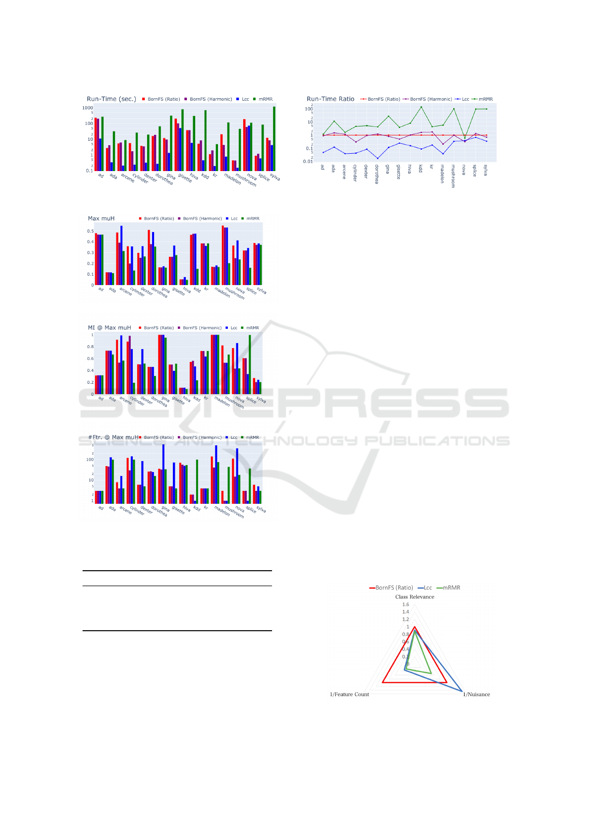
Figure 3: Run-time in logarithmic scale (iMac Pro with 2.5GHz 14-core Xeon W, averages of ten trials).

(a) Maximum µ

(F ;C).

(b) Class relevance: I(F ;C).

Figure 4: Results when µ

(F ;C) is maximized.

Table 2: Averaged ratios when µ

(F ;C) is maximized.

BORNFS

LCC mRMR

(F ;C) 1.00 0.90 1.06 0.76

I(F ;C) 1.00 0.92 0.91 0.87

H(F | C) 1.00 1.02 0.68 1.95

|F | 1.00 0.50 3.12 3.84

The observation is that LCC records low nui-

sance scores across datasets without considering nui-

sance in feature selection. Despite this, LCC selects

more features than others; for example, in the GINA

dataset, BORNFS selects around 30 features while

LCC chooses over 500.

The difference arises from the feature selection

methodologies. LCC uses a pre-established feature

order, leading to redundant feature selection. In con-

trast, BORNFS updates its feature order based on pre-

viously selected features, reducing redundancy and

creating a more streamlined feature set.

8 APPLICATION TO A HUGE

REAL DATASET

To assess BORNFS’s performance on large datasets,

experiments were conducted using the EMBER repos-

itory, intended to foster malware detection research.

The dataset includes over 10 million features and

comprises 300,000 benign and 300,000 malicious

samples for training, along with 100,000 of each for

testing.

Due to the massive feature count over 10 million,

a two-step approach was adopted for BORNFS to ef-

ﬁciently handle the dataset:

1. Initial Reduction: BORNFS was deployed with

h = ∞ and t = 1.0 on the complete dataset to

signiﬁcantly reduce the feature count. This step

likely leaves a substantial number of redundant

features.

2. Redundancy Elimination: To remove redundant

features from the initial reduction, BORNFS was

reapplied with h = 10 to the reduced feature set.

The threshold parameter t was varied among 1.0,

0.95, and 0.9 for this purpose.

Figure 5: Radar chart.

ICAART 2024 - 16th International Conference on Agents and Artiﬁcial Intelligence

1106

Table 3: Two-step application of BORNFS changing the hop

parameter values.

Initial h = ∞ h = 10

t = 1.0 t = 1.0 0.95 0.9

Feature count 10,868,073 541 540 155 50

AUC-ROC LGBM 0.97 0.97 0.96 0.86

AUC-ROC MLP 0.98 0.98 0.98 0.88

Runtime (min.) 24.33 515.92 69.09 9.57

To determine the predictive capability of the fea-

ture subsets from the two-step approach, LGBM and

MLP classiﬁers were used on the reﬁned dataset, and

AUC-ROC scores were calculated. Remarkably, with

the threshold parameter t at 0.95, AUC-ROC scores

were high, reaching 0.96 for LGBM and 0.98 for MLP,

despite reducing the feature count from over 10 mil-

lion to just 155. These results are detailed in Table 3.

The experiment was conducted on an AWS

r5.4xlarge instance, which has 16 vCPUs and 128GB

of memory. The total time taken for the experiment

with t = 0.95 was 93 minutes, comprising 24 minutes

for the ﬁrst step and an additional 69 minutes for the

second step.

9 CONCLUSION

Beyond the established metrics for evaluating the

goodness of feature selection, that is class relevance

and feature count, we introduced nuisance as a third

metric. This metric measures the amount of irrel-

evant data that can distort understanding. Our µ

score evaluates the balance between relevance and

nuisance and has shown a positive correlation with

classiﬁer performance. Our method, BORNFS, har-

monizes these metrics and has outperformed others,

including LCC and mRMR, on large datasets. It main-

tains accuracy while reducing the number of features.

ACKNOWLEDGEMENTS

This work was supported by JSPS KAKENHI Grant

Number 21H05052, and Number 21H03775.

REFERENCES

Almuallim, H. and Dietterich, T. G. (1994). Learning

boolean concepts in the presence of many irrelevant

features. Artiﬁcial Intelligence, 69(1 - 2).

Anderson, H. S. and Roth, P. (2018). EMBER: an open

dataset for training static PE malware machine learn-

ing models. CoRR, abs/1804.04637.

Blake, C. S. and Merz, C. J. (1998). UCI repository of ma-

chine learning databases. Technical report, University

of California, Irvine.

Hall, M. A. (2000). Correlation-based feature selection

for discrete and numeric class machine learning. In

ICML2000, pages 359–366.

KDD (1999). KDD Cup 1999: Computer network intrusion

detection.

Kira, K. and Rendell, L. (1992). A practical approach to

feature selection. In ICML1992, pages 249–256.

NIPS (2003). Neural Information Processing Systems Con-

ference 2003: Feature selection challenge.

Peng, H. (2007). mRMR (minimum Redundancy Maximum

Relevance Feature Selection. http://home.penglab.

com/proj/mRMR/. Online; accessed 29-February-

2020.

Peng, H., Long, F., and Ding, C. (2005). Fea-

ture selection based on mutual information: Cri-

teria of max-dependency, max-relevance and min-

redundancy. IEEE TPAMI, 27(8).

Shin K. and Maeda K. (2023). Temporarily open at.

https://00m.in/Xud17.

Shin, K., Fernandes, D., and Miyazaki, S. (2011). Consis-

tency measures for feature selection: A formal deﬁni-

tion, relative sensitivity comparison, and a fast algo-

rithm. In IJCAI2011, pages 1491–1497.

Shin, K., Kuboyama, T., Hashimoto, T., and Shepard, D.

(2015). Super-CWC and super-LCC: Super fast fea-

ture selection algorithms. In IEEE BigData 2015,

pages 61–67.

Shin, K., Kuboyama, T., Hashimoto, T., and Shepard, D.

(2017). sCWC/sLCC: Highly scalable feature selec-

tion algorithms. Information, 8(4).

WCCI (2006). IEEE World Congress on Computational In-

telligence 2006: Performance prediction challenge.

Yu, L. and Liu, H. (2003). Feature selection for high-

dimensional data: a fast correlation-based ﬁlter solu-

tion. In ICML2003.

Zhao, Z., Anand, R., and Wang, M. (2019). Maximum Rel-

evance and Minimum Redundancy Feature Selection

Methods for a Marketing Machine Learning Platform.

IEEE DSAA2019.

Zhao, Z. and Liu, H. (2007). Searching for interacting fea-

tures. In IJCAI2007, pages 1156 – 1161.

BornFS: Feature Selection with Balanced Relevance and Nuisance and Its Application to Very Large Datasets

1107