Transition of Model Performance in Dependence of the Amount of Data

Corruption with Respect to Network Sizes

Thomas Seidler

1,2 a

and Markus Abel

1,2 b

Ambrosys GmbH, Potsdam, Germany

Institute for Physics and Astronomy, Postsdam University, Potsdam, Germany

Keywords:

Phase Transition, Thermodynamics, Statistical Mechanics, Machine Learning, Image Classiﬁcation, MNIST.

Abstract:

An important question for machine learning model concerns the achievable quality or performance of a model

with respect to given data. In other words, we want to answer the question how robust a model is with respect

to perturbation of the data. From statistical mechanics, a standard way to ”corrupt” input data is a study that

uses additive noise to perturb data. This, in turn, corresponds to typical situations in processing data from any

sensor as measurement noise. Larger models will often perform better, because they are able to capture more

variance of the data. However, if the information content cannot be retrieved due to too large data corruptions

a large network cannot compensate noise effects and no performance is gained by scaling the network. Here

we study systematically the said effect, we add diffusive noise of increasing strength on a logarithmic scale

to some well-known datasets for classiﬁcation. As a result, we observe a sharp transition in training and test

accuracy as a function of the noise strength. In addition, we study if the size of a network can counterbalance

the described noise. The transition observed resembles a phase transition as described in the framework of

statistical mechanics. We draw an analogy between systems in statistical mechanics and Machine Learning

systems that suggests general upper bounds for certain types of problems, described as the tuple (data, model).

This is a fundamental result that may have large impact on practical applications.

1 INTRODUCTION

Any Machine Learning (ML) algorithm depends on

data as its input. The algorithm uses the input data

and transforms them to results which are ranked ac-

cording to a score. All data are limited in accuracy by

numerical accuracy, sensor noise, or noise in commu-

nication channels, etc.

Consequently, it is an important question to un-

derstand what amount of corruption an algorithm can

sustain, or at which noise level data corruption leads

to bad performance of a machine learning algorithm,

respectively. It is of equal importance to the optimal

model size needed for a successful training. We inves-

tigate both questions, inspired by the analogy of this

”coginition transition” and transitions as known from

physics - phase transitions and highlight how they are

related to one another in the light of statistical me-

chanics. To the best of our knowledge unveiling this

connection is a novel approach.

https://orcid.org/0000-0002-6870-5846

https://orcid.org/0000-0001-8963-6010

Statistical mechanics have been investigated in the

last decades (Bahri et al., 2020; Carleo et al., 2019;

ezard and Montanari, 2009) with strong reference

to early work on non-equilibrium thermodynamics of

learning (Gardner, 1988; Sompolinsky et al., 1990;

orgyi, 1990; Seung et al., 1992; Watkin et al.,

1993), and more recent advances by Biehl et al.

(2007), and Advani et al. (2013).

We relate our study of noise on data to phase tran-

sitions that occur with increasing/decreasing temper-

ature in statistical mechanics.

The paper is structured as follows: We provide a

more detailed account of the background in Sec. 2.

We present the method and data we use in Sec. 3.

In Sec. 4 we present the results we ﬁnd. In Sec. 5

and Sec. 6 we discuss the possible implications of our

ﬁndings and give an outlook to future directions of

study.

1084

Seidler, T. and Abel, M.

Transition of Model Performance in Dependence of the Amount of Data Corruption with Respect to Network Sizes.

DOI: 10.5220/0012435000003636

Paper published under CC license (CC BY-NC-ND 4.0)

In Proceedings of the 16th International Conference on Agents and Artiﬁcial Intelligence (ICAART 2024) - Volume 3, pages 1084-1091

ISBN: 978-989-758-680-4; ISSN: 2184-433X

2 BACKGROUND

The performance of Machine Learning models is in-

trinsically linked to the quality and quantity of data

used in training and inference (Cortes et al., 1994)

and the number of parameters in a model. The ef-

ﬁciency in terms of computational cost and speed is

furthermore related to mainly dataset and model size

(Al-Jarrah et al., 2015). With the advent of founda-

tional models, neural scaling laws, i.e. the scaling

of model performance with the amount of training

data and model size, have gained signiﬁcance (Kaplan

et al., 2020). It is therefore of crucial importance for

the practitioner to gauge the requirements for quality

and amount of data to train an ML model of a certain

size, and how much improvement in model perfor-

mance can be expected by adding more data or scal-

ing the model in order to work in a cost-effective and

sustainable manner.

Noise is a common source of data imperfections.

The impact of data corruptions on model performance

is reviewed by Drenkow et al. (2021). Large amounts

of noise are generally detrimental to model perfor-

mance. Noise originates from multiple sources, e.g.

sensor noise, transmission errors, and noise in the

signal source itself. Noise in image recognition is

often modeled as additive Gaussian noise (Boncelet,

2009). The addition of noise to data has recently

gained attention in the ﬁeld of generative, diffusion-

based models (Sohl-Dickstein et al., 2015; Ho et al.,

2020). These models are trained to de-noise im-

ages at varying intensities and subsequently generate

new images from the learned distribution, using pure

noise as input. The emphasis here is not on replicat-

ing real-world noise but on exploiting the statistical

properties of artiﬁcially introduced, controlled noise.

De-noising strategies and model architectures are re-

viewed by Tian et al. (2020), with notable applica-

tions found in Smilkov et al. (2017); Koziarski and

Cyganek (2017).

In statistical mechanics, noise is of thermal ori-

gin. Temperature drives phase transitions in (macro-

scopic) order parameters of ensembles of microscopic

constituents that are subject to thermal noise. A phase

transition is characterized by a sudden, in the limit of

inﬁnitely large systems (thermodynamic limit), dis-

continuous change in one or more order parameters or

their derivatives. Such transitions are typically driven

by (thermal) noise. Real-world systems display ﬁnite-

size effects, as they do not reach the thermodynamic

limit. Instead of a true discontinuity, the order pa-

rameter typically changes in a sigmoidal shape, with

the parametrization of the sigmoid depending on the

system size. These effects are governed by scaling

laws. For an introduction into statistical mechanics,

see Huang (2009).

Phase transitions have been found and studied in

numerous non-physical systems, e.g. in biology (Hef-

fern et al., 2021), in computer science (Martin et al.,

2001), in social science (Perc et al., 2017), and espe-

cially in the dynamics of learning (Seung et al., 1992;

Watkin et al., 1993; Carleo et al., 2019; Bahri et al.,

2020) to name but a few examples. In turn, ML mod-

els are used to identify phase transitions in several

physical systems, e.g. in quantum mechanics (Rem

et al., 2019), complex networks (Ni et al., 2019), and

condensed matter (Carrasquilla and Melko, 2017).

More general approaches to detecting phase transi-

tions using Machine Learning are found in Canabarro

et al. (2019); Giannetti et al. (2019); Suchsland and

Wessel (2018).

ML model performance is quantitatively assessed

using metrics that statistically summarize the infer-

ence on all (microscopic) data points in train, test,

and validation datasets. This macroscopic quantity is

essentially an order parameter as they are deﬁned in

statistical mechanics to describe systems with large

numbers of microscopic constituents. Especially in

classiﬁcation tasks the analogy to spin systems is evi-

dent; the accuracy of a classiﬁcation model describes

the average over a binary state variable, that is typi-

cally 1 for correct classiﬁcation on a data point and

either −1 or 0 for an incorrect classiﬁcation. In the

framework of statistical mechanics the dependence of

model performance on data quality (noise) is identi-

ﬁed as the dependence of an order parameter on tem-

perature in the statistical mechanics sense, and neural

scaling laws are analogous to the scaling laws related

to ﬁnite-size effects. We draw an analogy between

the sigmoidal decline of model performance with in-

creasing noise and phase transitions. However, this

analogy is limited. While phase transitions in physical

systems are driven by external ﬁelds and microscopic

dynamics, we here investigate the static performance

of ML models on training and test data.

3 METHODS AND DATA

In this section, we explain which data we use, and

how we study them. In essence, we require the data to

be large enough in number to allow for an investiga-

tion over several scales, and the task should be simple

enough to allow for statistically signiﬁcant noise vari-

ation, but complex enough to allow an extrapolation

for modern tasks in machine learning. We identiﬁed

image classiﬁcation as a good task with many known

and available datasets.

Transition of Model Performance in Dependence of the Amount of Data Corruption with Respect to Network Sizes

1085

Table 1: Summary of the features of the MNIST, Fashion-

MNIST (F-MNIST), and EMNIST (balanced) dataset.

MNIST F-MNIST EMNIST

number of 1797 70 000 131 600

images

classes 10 10 47

image size 8 ×8 28 ×28 28 ×28

3.1 Classiﬁcation Datasets

We study the inﬂuence of noise on the performance of

a network and the possible consequences on network

architecture or size in image classiﬁcation tasks.One

of the probably best-studied datasets is the MNIST

dataset (LeCun et al., 2010; Deng, 2012). How-

ever the dataset size is N

MNIST

≃ 10

3 1

which is too

small for a reasonable study over several scales and

considered ”too easy” to provide a basis for mean-

ingful studies (Xiao et al., 2017). The FashionM-

NIST dataset provides the same number of (balanced)

classes as MNIST and a similar amount of available

data but on downscaled greyscale images of fashion

items. The FashionMNIST benchmark studies (Xiao

et al., 2017) show that the classiﬁcation models for

fashion items generally achieve poorer performance

compared to the same model setups for handwritten

digits. For our purpose this is a deﬁning trait of a

dataset being more complex in terms of the classiﬁca-

tion task at hand. The EMNIST dataset (Cohen et al.,

2017) contains the MNIST data as a subset, but adds

other handwritten literals and contains more samples

per class, see Tab. 1. The added number of classes

in EMNIST further increases complexity (Baldomi-

nos et al., 2019), so we focus on the EMNIST data in

the further presentation.

Figure 1: EMNIST example image, belonging to class num-

ber 13 ( the letter ”H”).

In the aggregation that we use found in Tensorﬂow De-

velopment Team (2023)

3.2 Modeling Noise

Noise in realistic data can have many causes, and ex-

hibit complicated distributions in the noise signal; it

can be additive or multiplicative, and be subject to

very complex generation mechanisms (van Kampen,

1992).

For the EMNIST data, we have to consider that

the images have pixelwise greyscale values bounded

between 0 and 255. Naively, one might attempt to use

Gaussian noise of zero mean and varying variance to

control the intensity. That will result in essentially en-

larging the original domain of the data for large noise

additions.

One way out of the described dilemma is given

by recent developments, so-called denoising diffusion

probabilistic models (DDPM) (Sohl-Dickstein et al.,

2015), e.g. Stable Diffusion (Ho et al., 2020). In

the following, we outline the data corruption scheme

from (Ho et al., 2020), which is the sampling scheme

used in this study, to introduce some notation.

The rule for adding Gaussian noise to initial data

∈ R

to produce a corrupted data sample x

reads

= f (x

t−1

,γ

+ g(x

t−1

,β

)ε

(1)

Where β

, γ

are (series of) constants called a noise

schedule, ε is noise drawn from a Gaussian distribu-

tion with variance β

and 0 mean, and t denotes the

timestep in the Markov chain used to gradually add

noise. f (x

t−1

,γ

) can be interpreted as drift of the

mean, whereas g(x

t−1

,β

) governs the diffusion pro-

cess.

It can be shown that this formulation is equiva-

lent to using Markov transition kernels to transform

the prior distribution q(x

) to another distribution

) =

p(x

t−1

)p(x

t−1

)dx

t−1

with the proper

choices of the transition kernel p(x

t−1

) and sam-

pling from this transformed distribution.

Our goal is to approximate a well-known distri-

bution, in our case a Guassian of zero mean and unit

variance, while using a version of the original data

that is scaled to zero mean and unit variance in a pre-

processing step as ground truth.

We choose the transition kernel to be a Gaussian

conditioned via its mean on the prior value and utilize

a noise schedule {β

}

t∈(0,...,T )

such that the transition

kernel reads

p(x

t−1

) = N (x

;

1 −β

t−1

,β

I). (2)

We can the expand on the series of Markov transi-

tions to write

q(x

) = Π

t=0

N (x

;

1 −β

t−1

,β

I). (3)

ICAART 2024 - 16th International Conference on Agents and Artiﬁcial Intelligence

1086

Using the notation α

:= 1 −β

and

:= Πα

and

some basic calculus, we can deﬁne the closed form

distribution at timestep t as

q(x

) = N (x

;

√

(1 −

)I) (4)

Equivalently, the sampling can the be realized as

√

1 −

0,I

. (5)

The choice of variance schedule β needs to ensure

that

→0 for t >> 1 so that we approximate a Gaus-

sian distribution of zero mean and unit variance.

Note that σ :=

(1 −

) deﬁnes the standard de-

viation in the sampling scheme, while µ :=

√

scales

the mean value of the distribution. We will use

κ := σ/µ (6)

as a dimensionless parameter to indicate noise in-

tensity.

The noise schema described above achieves ex-

actly what we desire: A mapping between original

distribution and pure noise distribution (i.e. signal to

noise ratio κ

−1

→ 0 as t → T ) with a cheap sampling

scheme and conservation of the domain of the target

set.

The result of the process is depicted for two noise

levels in Fig. 2.

3.3 Experiment Design

This study investigates the robustness of feedforward

artiﬁcial neural networks by varying the number of

hidden units, and noise intensities in the data, to un-

derstand the transition from optimal model accuracy

to baseline accuracy (that is identical with guessing

the label for each image).

3.3.1 Model Architecture

We utilized a multilayer perceptron (MLP), a class of

feedforward artiﬁcial neural network. The MLP was

designed with an input layer, one hidden layer, and an

output layer. The hidden layer used the rectiﬁed linear

unit (ReLU) activation function, ensuring non-linear

transformations of the inputs. The output layer’s acti-

vation function was tailored to the nature of the task,

i.e. softmax for the classiﬁcation tasks.

For details on ML models and methods we refer

to Goodfellow et al. (2016).

3.3.2 Hyperparameters

Hyperparameters in machine learning typically re-

fer to non-trainable parameters of the model. How-

ever, in our experiment design, models and data are

Figure 2: EMNIST image with three different noise intensi-

ties added, top: κ = 46, middle: κ = 134, bottom: κ = 871.

constituents of one joint system. Especially the dis-

tribution of model performance is expected to be

parametrized by parameters that describe both models

and data. In this context, we refer to all non-trainable

parameters as hyperparameters in our experiments,

including noise intensity, but also ”classical” hyper-

parameters regarding the models that are trained, in-

cluding the model size.

We experimented with varying the number of hid-

den units in the MLP models, speciﬁcally testing con-

ﬁgurations with (2,4,8, 16,32, 64,128) units respec-

tively.

To evaluate the robustness of the MLP models

against noisy data, we introduced different intensi-

ties of noise into the datasets. They are characterized

by the κ value from the noise scheme, cf. Sec. 3.2.

This noise was artiﬁcially generated, simulating real-

world data imperfections. The noise schedule that

Transition of Model Performance in Dependence of the Amount of Data Corruption with Respect to Network Sizes

1087

was used is given by β

= β

+ (β

−β

)t/n

steps

with

= 0.0001, β

= 0.02, and n

steps

= 3000. We took

samples every 300 steps.

3.3.3 Training and Evaluation

The MLP models were trained using a backpropaga-

tion algorithm with the Adam optimizer, a variant of a

stochastic gradient descent. The models were trained

for a maximum of 200 epochs. Model performance

was evaluated using the accuracy score, given by

acc(y, ˆy) =

samples

∑

1( ˆy

= y

) (7)

where y is the predicted label, ˆy the true label, and

1(a,b) = 1 i f a = b, else 0 is the indicator function.

Other metrics, namely F1 score, precision, and re-

call on test and training datasets have been recorded as

well, but did not yield additional insights. To specif-

ically measure robustness, we measured the perfor-

mance of each model as a function of noise intensity.

Training of ML models is not necessarily deter-

ministic, as it depends on the random initialization

of weights, and in our case random noise on the data

which is newly sampled for each training run. Some

training algorithms are not fully deterministic as well,

e.g. stochastic gradient descent. Especially in the

regime of large noise it might well be the case that

no global but rather a local minimum is found in the

optimization. As such, the training and test metrics

in each training run have to be interpreted as random

variables, sampled from an unknown distribution that

can be parametrized by the hyperparameters of inter-

est.

We measure the ﬁrst and second moments of the

parametric family of distributions, i.e. averages and

standard deviations of training and test metrics. We

thus repeat the training for each set of hyperparame-

ters N

realizations

= 10 times, and refer to a single train-

ing run as a realization of the system.

3.3.4 Execution

All models were implemented using the scikit-learn

framework (Pedregosa et al., 2011), and parallelized

with the dask library (Dask Development Team,

2016). Experiments were run on the JUWELS com-

puting cluster, ensuring consistent and efﬁcient com-

putation. The combinatorics of model architectures

as well as noise intensities poses a practical challenge.

The study amounts to ≈800 training runs, consuming

O(10

) CPU-hours in total. In order to keep track of

all hyperparameters and metrics computed, the man-

tik platform (Seidler et al., 2023) was used for exper-

iment execution and tracking.

4 RESULTS

In this section, we describe results for the EMNIST

dataset to have a dataset large enough to avoid insuf-

ﬁcient results due to size. Notions of model perfor-

mance refer to the accuracy score. Qualitatively iden-

tical results have been observed for the F1-score.

Our study aims at determining scaling laws of

model performance with respect to size and identify-

ing phase transitions with respect to noise in the data.

In statistical mechanics, that amounts to mimic the

asymptotic limit N

net

7→ ∞, such that a discontinuous

transition is observed. For such a study, in statisti-

cal mechanics, one has to consider ﬁnite-size effects.

These effects are evident in the saturation of optimal

model performance with increasing model size.

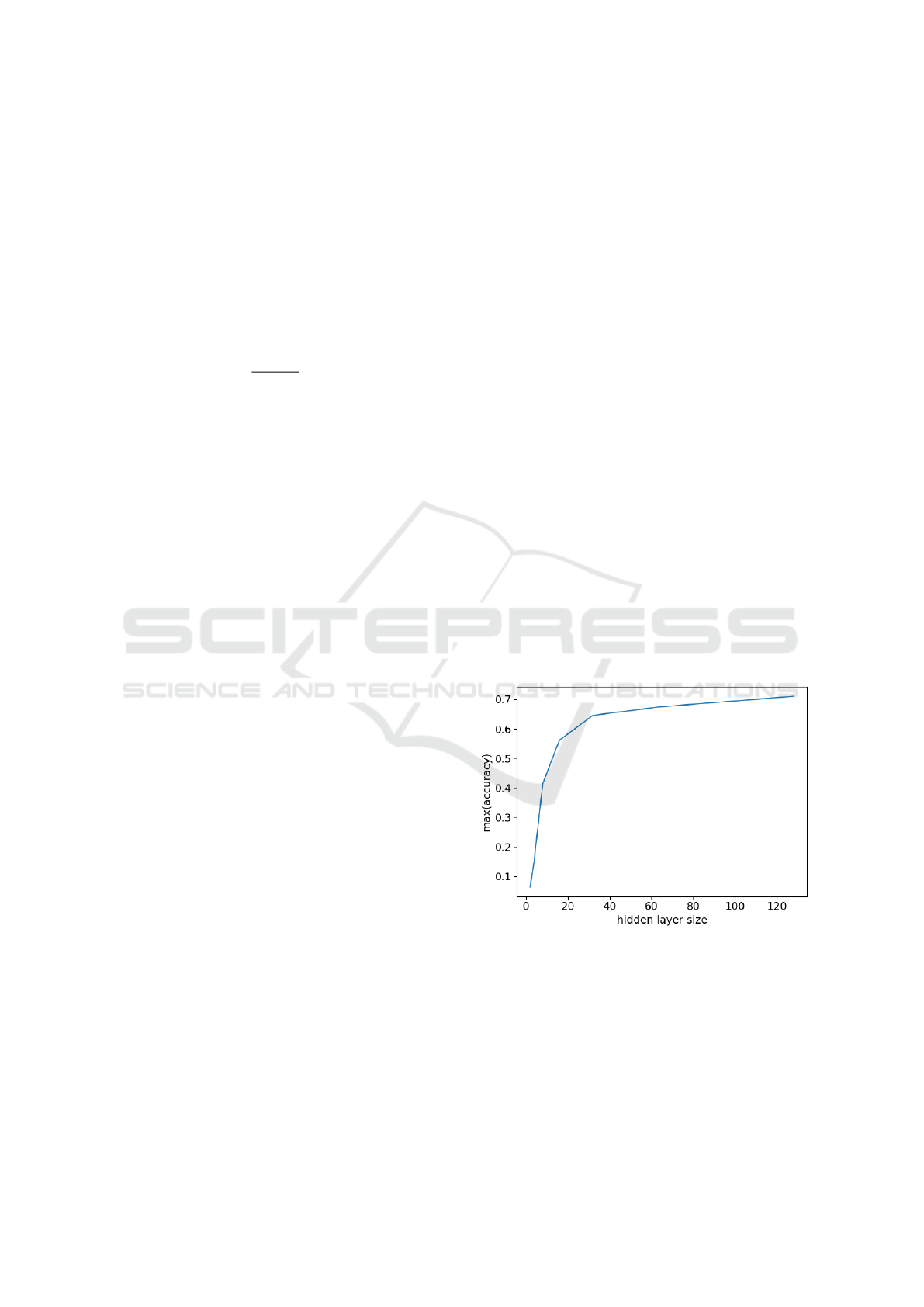
We study the convergence of the optimal accu-

racy achievable with multilayer perceptrons of vary-

ing size. In Fig. 3 we display the maximum test score

achieved with the perceptron model for increasing

size of the single layer used. We observe a conver-

gence and saturation for large N

net

. This is explained

by the relatively easy task to classify just N

classes

= 47

classes. with data of resolution N

pix

= 28x28. With

e.g. 128 neurons, we can capture O(2

128

) combina-

tions, and consequently much, if not all, of variance

of the images studied. So, we observe approximate

saturation at N

net

≃ 64, which is, again, characteristic

for the particular model and dataset studied.

Figure 3: Maximum test accuracy as a function of number

of hidden units in a feed forward neural network trained on

EMNIST data.

In Fig. 4, we show model performance as a func-

tion of noise for one very small network (N

network

= 2)

and one where the optimal performance approaches

saturation (N

network

= 128) as indicated in Fig. 3.

Clearly, overﬁtting occurs for larger network size in

the training, and smaller network size leads to the

expected incapability of the model to capture any

ICAART 2024 - 16th International Conference on Agents and Artiﬁcial Intelligence

1088

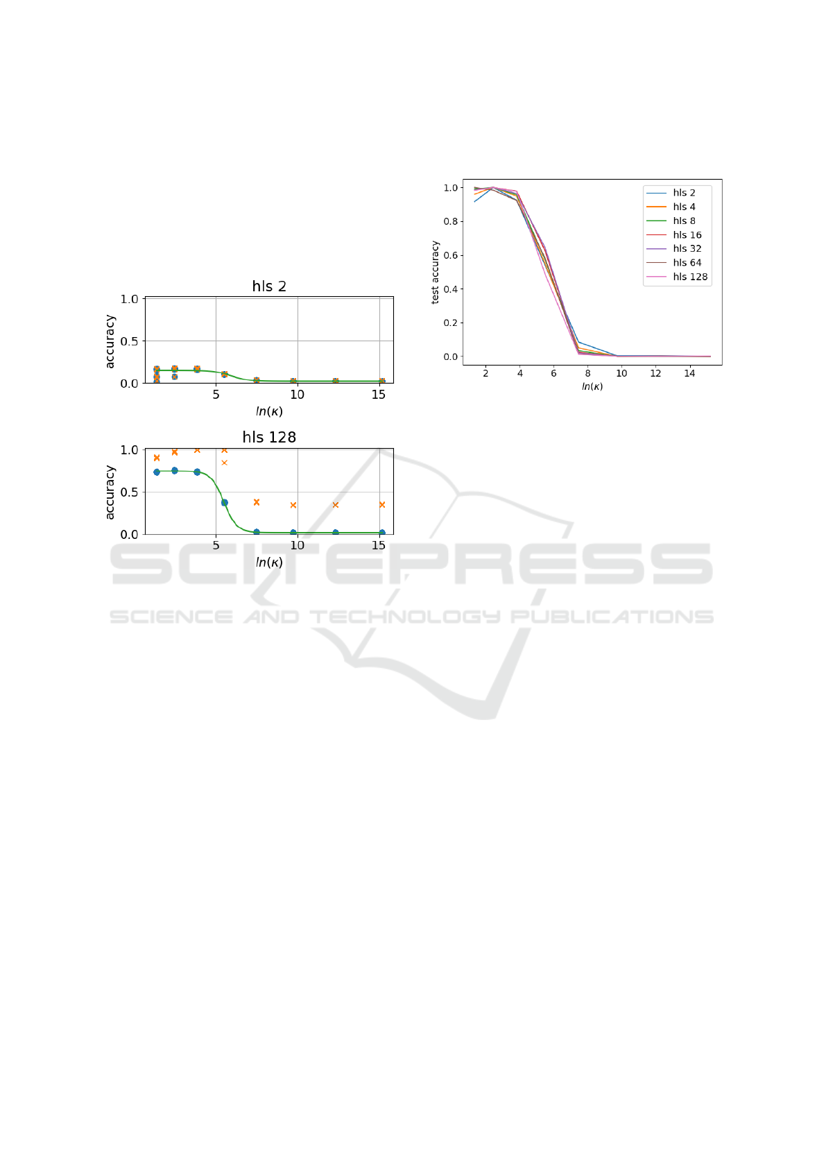
classiﬁcation. For the test data, we ﬁnd in all net-

work sizes a sigmoid-shaped transition with increas-

ing noise level. For the small network shown, with

network

= 2 we ﬁnd an upper bound for the test data

of accuracy acc = 0.2 (we start with an obviously

insufﬁcient number of nodes), while the larger net-

work with N

network

= 128 saturates at approximately

acc = 0.75 test accuracy for small noise intensity.

Figure 4: Test accuracy (blue circle), training accuracy (or-

ange cross), and sigmoidal ﬁt (green) as a function of noise

intensity for model sizes (hidden layer size hls = (2,128))

on the EMNIST dataset. The R

-score for the ﬁts are 0.82

for hls = 2, and > 0.99 for hls = 128 indicating that for the

larger model the data matches the sigmoid function very

well. Note that a too large model size causes overﬁtting

(training score= 1) but increase maximum test accuracy.

Phenomenologically, this resembles a phase tran-

sition, as it occurs in physics, e.g. in changes of state

from gas to liquid, magnetization, spin glasses - criti-

cal phenomena in general. We do not try to formally

map the small network with (with respect to the ther-

modynamic limit) small data.

In Fig. 5 we show the results for N

net

2,4, 8,16,32,64,128, where we have scaled the accu-

racy to minimum 0 and maximum 1. As discussed

above this is necessary because for small network

size, the maximum accuracy decreases. Remarkably,

the scaled curves overlap nicely, indicating that the

transition can be modeled by the same family of func-

tions regardless of network size. In Fig. 4 we show

that the transition has sigmoidal shape. Note that the

results are special to the investigated model (multi-

layer perceptron) and data (EMNIST), and the ques-

tion in how far the result is universal remains open

until we have studied a large set of models for dif-

ferent datasets, starting with different models for the

EMNIST data.

Figure 5: Maximum accuracy score out of the N

realizations

10 realizations as a function of logarithm of noise intensity

κ, normalized to maximum overall scores, for all studied

model sizes (hidden layer size hls).

5 CONCLUSION

We investigate the question in how far the transition

observed above is general. In the context of statisti-

cal mechanics, we want to understand i) whether the

transition point is universal for the data studied, or

the model used. We would expect that more elaborate

models do not only classify with better accuracy, but

also be able to account for more noise in the data; ii)

whether the transition shape is universal for different

models; iii) whether the transition (shape and point)

does depend on the noise, i.e. if Gaussian noise has

different results than uniformly distributed noise or

exponentially or spatially varying one.

As a starting point, we have studied one dataset

with one particular model, and therein we have varied

the network size in a controlled way - the model was

deliberately chosen to be simple and understandable

before we step to more general investigations.

We have shown that the analogy to the phe-

nomenology of phase transitions can be applied to es-

timate model robustness to noise in the data and un-

derstand scaling of model performance with model

size. However, we have focused on the task of im-

age classiﬁcation and investigated only datasets that

are closely related to one another. While this was

necessary in order to have controlled experimentation

conditions, it is favorable to deﬁne measures that are

intrinsic to data and models, i.e. intrinsic to the prob-

ability densities involved, without having to rely on

speciﬁc choices of metrics or noise.

Transition of Model Performance in Dependence of the Amount of Data Corruption with Respect to Network Sizes

1089

6 OUTLOOK

Further studies will focus on scaling of the observed

phenomena with the size of the dataset - a very impor-

tant question for real applications and related to en-

ergy saving and sustainability questions. It may well

be that for certain data it is useless to increase the size

of the data, because model performance is already in

saturation. Further, we will study the shape of the

transition in detail for a statistically representative set

of models, e.g. CNN vs. RNN vs. perceptrons. Lastly

we will extend the study to more diverse datasets.

Information theory provides deﬁnitions and inter-

pretations of quantities also known in statistical me-

chanics, such as entropy, in a way that is readily us-

able in the context of our experiments. A future goal

concerns theoretical work on universality of phase

transitions and scaling laws for (model, data) tuples

and their representation with respect to given tasks,

like classiﬁcation and regression. The goal is to uni-

versally compare models and datasets to one another

with respect to robustness, to infer both dataset com-

plexity and model robustness, ultimately deﬁning uni-

versality classes, as are well known from the theory of

phase transitions.

Eventually, we expect that studies on the ﬁnite size

effect, i.e. little data and/or small networks play a cru-

cial role. Our ﬁnal aim is to provide a tool to deter-

mine the optimum network size and data size for a

problem given, in particular when data quality is un-

known.

ACKNOWLEDGEMENTS

We acknowledge fruitful discussions with F. Em-

merich, M. Quade, and M. Schultz. This work is sup-

ported by the KI:STE project, grant no. 67KI2043 by

the German ministry for ecology. This research was

supported in part by the National Science Foundation

under Grant No. NSF PHY-1748958.

REFERENCES

Advani, M., Lahiri, S., and Ganguli, S. (2013). Statisti-

cal mechanics of complex neural systems and high

dimensional data. Journal of Statistical Mechanics:

Theory and Experiment, 2013(03):P03014.

Al-Jarrah, O. Y., Yoo, P. D., Muhaidat, S., Karagiannidis,

G. K., and Taha, K. (2015). Efﬁcient machine learning

for big data: A review. Big Data Research, 2(3):87–

93. Big Data, Analytics, and High-Performance Com-

puting.

Bahri, Y., Kadmon, J., Pennington, J., Schoenholz, S. S.,

Sohl-Dickstein, J., and Ganguli, S. (2020). Statistical

mechanics of deep learning. Annual Review of Con-

densed Matter Physics, 11:501–528.

Baldominos, A., Saez, Y., and Isasi, P. (2019). A survey

of handwritten character recognition with MNIST and

EMNIST. Applied Sciences (Switzerland), 9.

Biehl, M., Ahr, M., and Schl

osser, E. (2007). Statistical

physics of learning: Phase transitions in multilayered

neural networks. Advances in Solid State Physics 40,

pages 819–826.

Boncelet, C. (2009). Chapter 7 - Image Noise Models. In

Bovik, A., editor, The Essential Guide to Image Pro-

cessing, pages 143–167. Academic Press, Boston.

Canabarro, A., Fanchini, F. F., Malvezzi, A. L., Pereira, R.,

and Chaves, R. (2019). Unveiling phase transitions

with machine learning. Phys. Rev. B, 100:045129.

Carleo, G., Cirac, I., Cranmer, K., Daudet, L., Schuld,

M., Tishby, N., Vogt-Maranto, L., and Zdeborov

a, L.

(2019). Machine learning and the physical sciences.

Reviews of Modern Physics, 91:045002.

Carrasquilla, J. and Melko, R. G. (2017). Machine learning

phases of matter. Nature Physics, 13(5):431–434.

Cohen, G., Afshar, S., Tapson, J., and Schaik, A. V. (2017).

EMNIST: Extending MNIST to handwritten letters.

Proceedings of the International Joint Conference on

Neural Networks, 2017-May.

Cortes, C., Jackel, L. D., and Chiang, W.-P. (1994). Limits

on learning machine accuracy imposed by data qual-

ity. Advances in Neural Information Processing Sys-

tems, 7.

Dask Development Team (2016). Dask: Library for dy-

namic task scheduling.

Deng, L. (2012). The mnist database of handwritten digit

images for machine learning research. IEEE Signal

Processing Magazine, 29:141–142.

Drenkow, N., Sani, N., Shpitser, I., and Unberath, M.

(2021). A systematic review of robustness in deep

learning for computer vision: Mind the gap? arXiv

preprint arXiv:2112.00639.

Gardner, E. (1988). The space of interactions in neural net-

work models. Journal of Physics A: Mathematical and

General, 21(1):257.

Giannetti, C., Lucini, B., and Vadacchino, D. (2019). Ma-

chine learning as a universal tool for quantitative in-

vestigations of phase transitions. Nuclear Physics B,

944:114639.

Goodfellow, I., Bengio, Y., and Courville, A. (2016). Deep

Learning. MIT Press. http://www.deeplearningbook.

org.

orgyi, G. (1990). First-order transition to perfect gen-

eralization in a neural network with binary synapses.

Physical Review A, 41(12):7097–7100.

Heffern, E., Huelskamp, H., Bahar, S., and Inglis, R. F.

(2021). Phase transitions in biology: From bird ﬂocks

to population dynamics. Proceedings of the Royal So-

ciety B: Biological Sciences, 288.

Ho, J., Jain, A., and Abbeel, P. (2020). Denoising diffusion

probabilistic models. Advances in Neural Information

Processing Systems.

ICAART 2024 - 16th International Conference on Agents and Artiﬁcial Intelligence

1090

Huang, K. (2009). Introduction to Statistical Physics, Sec-

ond Edition. Taylor & Francis.

Kaplan, J., McCandlish, S., Henighan, T., Brown, T. B.,

Chess, B., Child, R., Gray, S., Radford, A., Wu, J., and

Amodei, D. (2020). Scaling laws for neural language

models. CoRR, abs/2001.08361.

Koziarski, M. and Cyganek, B. (2017). Image recognition

with deep neural networks in presence of noise – deal-

ing with and taking advantage of distortions. Inte-

grated Computer-Aided Engineering, 24:1–13.

LeCun, Y., Cortes, C., and Burges, C. J. (2010). MNIST

handwritten digit database. ATT Labs [Online]. Avail-

able: http://yann.lecun.com/exdb/mnist, 2.

Martin, O. C., Monasson, R., and Zecchina, R. (2001).

Statistical mechanics methods and phase transitions

in optimization problems. Theoretical Computer Sci-

ence, 265(1):3–67. Phase Transitions in Combinato-

rial Problems.

ezard, M. and Montanari, A. (2009). Information,

Physics, and Computation. Oxford University Press.

Ni, Q., Tang, M., Liu, Y., and Lai, Y.-C. (2019). Machine

learning dynamical phase transitions in complex net-

works. Phys. Rev. E, 100:052312.

Pedregosa, F., Varoquaux, G., Gramfort, A., Michel, V.,

Thirion, B., Grisel, O., Blondel, M., Prettenhofer,

P., Weiss, R., Dubourg, V., Vanderplas, J., Passos,

A., Cournapeau, D., Brucher, M., Perrot, M., and

Duchesnay, E. (2011). Scikit-learn: Machine learning

in Python. Journal of Machine Learning Research,

12:2825–2830.

Perc, M., Jordan, J. J., Rand, D. G., Wang, Z., Boccaletti, S.,

and Szolnoki, A. (2017). Statistical physics of human

cooperation. Physics Reports, 687.

Rem, B., K

aming, N., Tarnowski, M., Asteria, L.,

aschner, N., Becker, C., Sengstock, K., and Weiten-

berg, C. (2019). Identifying quantum phase transitions

using artiﬁcial neural networks on experimental data.

Nature Physics, 15:1.

Seidler, T., Emmerich, F., Ehlert, K., Berner, R., Nagel-

Kanzler, O., Schultz, N., Quade, M., Schultz, M. G.,

and Abel, M. (2023). Mantik: A workﬂow plat-

form for the development of artiﬁcial intelligence on

high-performance computing infrastructures. Submit-

ted for publication to Journal of Open Source Soft-

ware September 2023.

Seung, H. S., Sompolinsky, H., and Tishby, N. (1992). Sta-

tistical mechanics of learning from examples. Physi-

cal Review A, 45:6056–6091.

Smilkov, D., Thorat, N., Kim, B., Vi

egas, F. B., and Wat-

tenberg, M. (2017). Smoothgrad: removing noise by

adding noise. CoRR, abs/1706.03825.

Sohl-Dickstein, J., Weiss, E. A., Maheswaranathan, N., and

Ganguli, S. (2015). Deep unsupervised learning using

nonequilibrium thermodynamics. 32nd International

Conference on Machine Learning, ICML 2015, 3.

Sompolinsky, H., Tishby, N., and Seung, H. S. (1990).

Learning from examples in large neural networks.

Phys. Rev. Lett., 65:1683–1686.

Suchsland, P. and Wessel, S. (2018). Parameter diagnos-

tics of phases and phase transition learning by neural

networks. Phys. Rev. B, 97:174435.

Tensorﬂow Development Team (2023). TensorFlow

Datasets, a collection of ready-to-use datasets. https://

www.tensorﬂow.org/datasets. Accessed: 13.11.2023.

Tian, C., Fei, L., Zheng, W., Xu, Y., Zuo, W., and Lin, C.-

W. (2020). Deep learning on image denoising: An

overview. Neural Networks, 131:251–275.

van Kampen, N. (1992). Stochastic Processes in Physics

and Chemistry. Elsevier Science Publishers, Amster-

dam.

Watkin, T. L., Rau, A., and Biehl, M. (1993). The statisti-

cal mechanics of learning a rule. Reviews of Modern

Physics, 65.

Xiao, H., Rasul, K., and Vollgraf, R. (2017). Fashion-

MNIST: a Novel Image Dataset for Benchmark-

ing Machine Learning Algorithms. arXiv preprint

arXiv:1708.07747.

Transition of Model Performance in Dependence of the Amount of Data Corruption with Respect to Network Sizes

1091