Serial or Simultaneous? Possible Attack Strategies with an Arsenal of

Attack Tools

Yahel Giat

and Irit Nowik

Department of Industrial Engineering, Jerusalem College of Technology, Havaad Haleumi 21, Jerusalem, Israel

Keywords:

Sequential, Parallel, Pooling, Cyber, Optimization.

Abstract:

In various ﬁelds such as medicine, management, cyber operations, and military strategy, the choice between

sequential and parallel strategies is pivotal in achieving objectives, be it maximizing the likelihood of success

or minimizing the time to victory. This study considers a hacker who attempts to destroy a rival system using

multiple attacking tools. It is assumed that the success probability of each attack tool to destroy the system

is equal and independent of the other tools. Execution of an attack is time consuming and it is assumed that

this attack time increases exponentially with the number of tools used simultaneously. We consider different

attaching schemes that vary in their design and balance between parallel and sequential steps. Our ﬁndings

indicate that when the attack time for a multi-tool attack is extremely short, the optimal solution will be a

purely simultaneous attack. Conversely, if the attack time approaches the total time required for a sequential

attack, then the optimal solution will be a purely sequential approach. In between these extremes, we discover

that a mixed strategy is optimal. Interestingly, our numerical analysis reveals that in these mixed cases, it is

consistently more advantageous to initiate a simultaneous attack and then complement it with a sequential one.

Moreover, we demonstrate that as the probability of success increases, the optimum tends towards a sequential

attack.

1 INTRODUCTION

In the realms of many disciplines such as medicine,

management, cyber and military operational art, the

choice between sequential and parallel strategies

plays a crucial role in achieving objectives, whether

its maximizing the probability of success or minimiz-

ing the time until victory. A sequential strategy in-

volves using the available tools one at a time, pro-

gressing to the next only if the previous one fails. In

contrast, a parallel strategy entails the employment of

many or all available tools simultaneously in a con-

certed effort.

Practical examples to this choice are abundant.

In the ﬁeld of medicine, for example, an oncologist

may ﬁnd that her patient’s tumor responds to only two

types of chemotherapies. Should she treat with both

simultaneously to maximize the chance of full tumor

lysis before the tumor develops defensive mutations?

Or perhaps, she should begin with monotherapy so

that in the event the tumor develops immunity to it,

she has another viable treatment for her patient. In

https://orcid.org/0000-0001-7296-8852

https://orcid.org/0000-0003-0697-8862

certain ﬁelds of medicine, a mix of simultaneous and

sequential strategies have been developed. For exam-

ple, physicians treating HIV carriers have recognized

as early as 1995 that a cocktail of drugs has better

results than sequential monotherapy, and when a spe-

ciﬁc cocktail is less effective then another cocktail is

used (Lu et al., 2018). Thus, both a simultaneous and

sequential approach are used.

This question has intrigued many thinkers in the

ﬁeld of combat and military. For example, Soucy

(2018) studies General MacArthur’s sequential ap-

proach against the Japanese in the South West Pa-

ciﬁc during World War II, and compares it with Gen-

eral Schwarzkopf’s parallel war against Iraq during

Desert Storm. His conclusion is that due to the

Unites State’s considerable military power, a parallel

war is advantageous and allows it to “quickly shatter

an enemy’s strategic and operational ability to resist

(Soucy, 2018, p. 3)”.

In this paper, we consider a hacker trying to attack

and destroy a system. The hacker has at its disposal

a pool of attack tools, whereas the attacked system

can (with a known probability) withstand an attack by

any one of the tools and develop defense mechanisms

Giat, Y. and Nowik, I.

Serial or Simultaneous? Possible Attack Strategies with an Arsenal of Attack Tools.

DOI: 10.5220/0012433800003639

Paper published under CC license (CC BY-NC-ND 4.0)

In Proceedings of the 13th International Conference on Operations Research and Enterprise Systems (ICORES 2024), pages 171-178

ISBN: 978-989-758-681-1; ISSN: 2184-4372

171

that allow it to be immune to that speciﬁc tool. This

setting gives rise to multiple attack strategies rang-

ing from fully sequential attacks (i.e., in each period a

single tool is employed until the system is destroyed),

to purely simultaneous attack in which all the attack

tools are used simultaneously. In between these two

extremes there are strategies that mix the sequential

and simultaneous approaches in varying degrees.

In our model, we assume that the probability of

success of each tool is equal and independent of the

other tools and show that if the attack time is inde-

pendent of the number of tools employed in the at-

tack, then the purely simultaneous strategy is optimal

to the hacker. In contrast, if attack time is the sum of

the individual attack times of the tools that it employs,

then the fully sequential strategy is optimal.

When attack time is increasing concavely with the

number of tools then strategies that mix between si-

multaneous and sequential attacks can be optimal, de-

pending on the total number of tools available to the

hacker and the probability of each tool to succeed.

While our model is quite simplistic in its nature,

it provides insights that may be useful whenever there

are multiple resources available. Staggering resources

in contrast to pooling them in a concerted effort is

of interest in a large array of applications, including

military, cyber, health and managerial.

2 LITERATURE REVIEW

Sequential versus simultaneous strategies have been

considered in a wide range of scientiﬁc ﬁelds. In

computer science, Andrad

ottir et al. (2017) studies a

model in which queues or servers may be pooled. It is

well known that pooling queues and servers is advan-

tageous when servers are not subject to failure. How-

ever, when servers could fail, then there is a tradeoff

between efﬁciency (queue length) and risk (i.e., the

probability that a system will be overcrowded). See

also Sunar et al. (2021) who considers a similar prob-

lem with different constraints. Similarly, Cui et al.

(2018) compares between simultaneous attacks and

sequential attacks on cyber-physical systems.

Sequential strategies are often likened to a cau-

tious approach and are widely used in the medical

ﬁeld, where the progression of treatment options de-

pends on patient response. A notable example of se-

quential strategy in medicine is the management of

cancer. Oncologists often begin with less aggressive

treatments, such as radiation therapy or chemother-

apy, and only switch to more invasive procedures like

surgery if the initial methods do not yield the de-

sired results. This approach minimizes the imme-

diate risks and side effects while keeping more po-

tent interventions in reserve but in some cases may

be more susceptible to mutants. For example, with

metastatic breast cancer, international guidelines rec-

ommend using sequential monotherapy unless there

is rapid disease progression (Cardoso et al., 2014).

A systematic review comparing between combina-

tion (i.e., simultaneous) and sequential therapy found

that there was no difference in overall survival be-

tween the two groups but found that when drugs were

given one at a time there may be more time before

the tumors grew back again thereby achieving longer

progression-free survival (Dear et al., 2013). In con-

trast, for the initial treatment of hypertension Mac-

Donald et al. (2017) found that combination therapy

is superior to sequential monotherapy. Another inter-

esting example is the medical management of patients

that are HIV positive. It is a long standing consensus

that a combination therapy is superior to sequential

monotherapy in stopping these patients from acquir-

ing AIDS (Lu et al., 2018). Despite this established

clinical approach, it has been suggested that certain

HIV subpopulations that are resistant to multi-drug

treatment may beneﬁt from a sequential monotreat-

ment approach (Phillips et al., 2003).

Sequential and parallel strategies also have a place

in the ﬁeld of management, where the objective is of-

ten to maximize business performance or minimize

operational challenges (e.g, Thompson and Kwort-

nik Jr, 2008). The sequential approach is frequently

employed when tackling complex problems or imple-

menting organizational changes (Read et al., 2001).

Managers may choose to take one step at a time, eval-

uating the effectiveness of each action before pro-

ceeding to the next. For instance, when faced with

declining proﬁts, a company may ﬁrst focus on cost-

cutting measures, followed by rebranding, and subse-

quently, market expansion. This sequential strategy

allows for a more measured evaluation of each phase

of the plan. Parallel strategies in management are of-

ten associated with rapid and comprehensive changes.

For instance, during a business turnaround, a com-

pany on the brink of failure may implement a com-

bination of cost-cutting measures, diversiﬁcation, re-

branding, and fundraising simultaneously to expedite

a recovery. This approach aims to address multiple

critical issues concurrently, potentially leading to a

quicker turnaround, but it also involves higher risk

and resource allocation Xiong et al. (2019).

Strategic planning is a framework used in various

sectors, including business, government, and the mil-

itary, with the primary goal of achieving long-term

objectives. For instance, during a military campaign,

a parallel approach might involve deploying all avail-

ICORES 2024 - 13th International Conference on Operations Research and Enterprise Systems

172

able resources, such as ground forces, air support, and

electronic warfare, in a coordinated effort to achieve a

swift and overwhelming victory. This approach seeks

to minimize the time until winning by overwhelming

the adversary. This approach is often evident in large-

scale offensives, where all available resources are de-

ployed simultaneously to overwhelm the enemy. The

“shock and awe” strategy, for example, aims to inca-

pacitate the adversary through a concentrated and si-

multaneous show of force (McNaughton, 2019). This

parallel approach can be highly effective in achieving

a swift victory but comes with higher risks and re-

source commitment. Conversely, a sequential military

strategy is often employed when precision and limited

collateral damage are essential. Surgical strikes con-

ducted by special forces units exemplify this approach

(Sasikumar, 2019).

The choice between sequential and parallel strate-

gies in medicine, management, and strategic plan-

ning depends on the speciﬁc objectives, risks, and re-

sources available. Each approach has its merits and

drawbacks, and a balanced combination of both may

be the most effective solution in many cases. Context-

speciﬁc analysis is essential to determine the optimal

strategy that will either maximize the winning proba-

bility or minimize the time until winning, depending

on the situation at hand.

3 THE BASIC MODEL

The environment that we present comprises two rival

entities. The attacking entity (“the hacker”) desires

to eliminate a system (“the system”) that the hacked

entity (“the hacked”) has acquired. To do so, the

hacker has at its disposal N distinct attack tools, each

of which can potentially eliminate the system. The

system has a lifespan of T periods after which it is

obsolete. Therefore, if all the attacks on it fail, it is

expected to survive exactly T periods.

The probability of each attack tool to successfully

eliminate the system is q and independently of the

other attack tools. In this case, we assume that the

system is eliminated at the end of the period. If the

attack tool fails to eliminate the system, it is assumed

that the attacked system was either prepared or has

developed defences against this tool and therefore this

attack tool is rendered useless.

In the basic model we assume that the attack time

is exactly one period regardless of the number of tools

employed. That is, an attack using one tool and at-

tack using k > 1 tools will each require one period to

set up. In the next section we relax this assumption.

Consider N strategies. Strategy Q

, k = 0, ..., N − 1

follows the subsequent steps:

1. Initialization: Success:=False, Pool:= N attack

tools.

2. Serial Phase: For j := 1, ...k

(a) In each period, attack with a single attack tool

from the pool of tools.

(b) Remove this tool from the pool.

Go to step 4.

3. Simultaneous Phase: In period k + 1 attack simul-

taneously with N − k (remaining) attack tools. If

successful Success:=True.

4. Output: Success.

Notice that strategy Q

, will last at most k + 1 periods

and that when k = 0 or k = N − 1 the strategies are

either purely simultaneous (k = 0) or only sequential

(k = N − 1).

In Figure 1 we depict the strategy Q

when N = 5.

The hacker attacks in the ﬁrst period with a single at-

tack tool. If this attack has succeeded then the sys-

tem’s survival was one period. Otherwise, the hacker

attacks again with another single tool, and if this at-

tack has succeeded then the system’s survival was two

periods. Otherwise, the hacker goes all in with the

three remaining tools at its disposal. If this simulta-

neous attack has succeeded then the system’s survival

was 3 periods and if not then the system’s survival

was T periods.

n = 0





tool 1

success

prob = q

survival =1

fail

prob = 1−q





tool 2

success

prob = q

survival = 2

fail

prob = 1−q





tools

3,4,5

success

prob = 1−(1−q)

survival = 3

fail

prob = (1−q)

survival = T

Figure 1: The Q

strategy in the basic model when N = 5

attacking tools are available.

Serial or Simultaneous? Possible Attack Strategies with an Arsenal of Attack Tools

173

Denote X as the random variable representing the

survival (i.e., length of life) of the attacked system.

The expected value of X comprises three elements.

First, it must survive the sequential phase. The sys-

tem is eliminated after j periods, 1 ≤ j ≤ k, if and

only if it survived the ﬁrst j − 1 periods, but was suc-

cessfully attacked in the jth period. The probability

for this to happen is (1−q)

j−1

q and when this hap-

pens the system survived exactly j periods. Thus, the

sequential phase contributes to the system’s expected

survival

∑

j=1

j(1−q)

j−1

q. The ﬁrm survives exactly

k + 1 units of time if the sequential phase failed, but

the simultaneous phase (that comprises N −k attack

tools) was successful. The probability of this is

(1−q)

(1−(1−q)

N−k

) = (1−q)

− (1−q)

and therefore the contribution of the simultaneous

phase to the expected survival is (k+1)



(1−q)

−(1−



. Finally, the system survives all the attacks with

probability (1 − q)

in which case it survives T peri-

ods and therefore this contributesT (1−q)

to the sys-

tem’s expected survival. Thus, the system’s expected

survival when strategy Q

is employed is given by:

= q

∑

j=1

j(1−q)

j−1

+ (k+1)



(1−q)

− (1−q)



+ T (1−q)

(1)

Lemma 1. The expected survival is increasing with

Proof. To show that a higher k results with longer sur-

vival we must show that for each k<N−1, it holds that

k+1

− E

> 0. By (1),

k+1

− E

= q(k + 1)(1−q)

(k+2)(1−q)

k+1

(1−(1−q)

N−k−1

)

− (k+1)(1−q)

(1−(1−q)

N−k

). (2)

Expanding the latter expressions gives

k+1

− E

= q(k + 1)(1−q)

(k+2)(1−q)

k+1

− (k+2)(1−q)

− (k+1)(1−q)

, (3)

which can be simpliﬁed to

k+1

− E

= q(k + 1)(1−q)

− (1−q)

(k+2)(1−q)

k+1

− (k+1)(1−q)

. (4)

The ﬁrst and fourth terms above can be combined to

−(k+1)(1−q)

k+1

and when added to the third term

results with (1−q)

k+1

. Therefore, (4) simpliﬁes to

k+1

− E

= (1 − q)

k+1

− (1 − q)

, (5)

which is positive since k + 1 < N.

Lemma 1 implies that the more the strategy is si-

multaneous (i.e, shorter sequential phase) the better

for the hacker. In fact, under the assumptions of the

basic model the best strategy is the pure simultane-

ous strategy, Q

. This result follows from the fact

that there is no probabilistic loss from attacking si-

multaneously (since the probabilities for success of

each attack tool are independent) whereas time-wise

a simultaneous approach is advantageous since more

attack tools are employed in a shorter time. In the

next section, we revisit this feature of the model con-

cerning the time that the hacker needs to execute a

simultaneous attack. In addition, we extend the menu

of strategies that we consider to strategies that begin

with a simultaneous attack employing a subset of the

tools followed by sequential attacks using the remain-

ing tools.

4 GENERALIZED MODEL

We consider two extensions to the model described in

the previous section.

4.1 Exponential Attack Time

The attack time for simultaneous cyber attacks may

not increase at a constant rate with the number of

attacking tools due to a concept known as “decreas-

ing marginal cost”. This idea comes from economics

and refers to the phenomenon where the cost of pro-

ducing each additional unit of a good or service de-

creases as the overall quantity increases. In the con-

text of cyber attacks, think of each attacking tool as a

unit. As you add more tools, there may be synergies

or efﬁciencies gained in the overall attack execution

process. For example, some tools may share com-

mon requirements or dependencies, and once those

are set up, adding more tools becomes quicker and

less resource-intensive.

Additionally, attackers may develop scripts or au-

tomated processes that can be reused across different

tools, further reducing the attack time for each addi-

tional tool. This is similar to economies of scale in

manufacturing, where producing more units leads to a

lower cost per unit. In line with these ideas we assume

that the attack time for a simultaneous attack with k

tools is k

, where α satisﬁes; 0 ≤ α ≤ 1. Note that

when α = 0, the attack time is constant in the number

of attacking tools, which is consistent with the basic

model (see Section 3), whereas α = 1 assumes that

the attack time is linear in the number of attackers

(i.e., the attack time increases at a constant rate with

the number of attacking tools). In Figure 2 we de-

ICORES 2024 - 13th International Conference on Operations Research and Enterprise Systems

174

pict the strategy Q

when N = 5. The hacker attacks

in the ﬁrst period with a single attack tool. If this at-

tack has succeeded then the system’s survival was one

period. Otherwise, the hacker attacks again with an-

other single tool, and if this attack has succeeded then

the system’s survival was two periods. Otherwise, the

hacker goes all in with the three remaining tools at

its disposal. If this simultaneous attack has succeeded

then the system’s survival was 2 + 3

periods and if

not then the system’s survival was T periods.

n = 0





tool 1

success

prob = q

survival =1

fail

prob = 1−q





tool 2

success

prob = q

survival = 2

fail

prob = 1−q





tools

3,4,5

success

prob = 1−(1−q)

survival = 2 + 3

fail

prob = (1−q)

survival = T

Figure 2: The Q

strategy in the Exponential model when

N = 5 attacking tools are available.

4.2 Simultaneous-Sequential Strategies

In Section 3 and 4.1 we considered a class of strate-

gies {Q

}, in which the hacker begins with a sequen-

tial approach and then delivers a ﬁnal simultaneous

attack. We now extend our consideration to include a

class of strategies {M

}, with this order reversed.

Strategy M

, k = 0, ..., N − 1 follows the subse-

quent steps:

1. Initialization: Success:=False, Pool:= N attack

tools.

2. Simultaneous Phase:

(a) For (N − k )

periods attack simultaneously

with N − k attack tools.

(b) Remove these tools from the pool.

Go to step 4.

3. Serial Phase: For j := 1, ...k

(a) In each period, attack with a single attack tool

from the pool of tools.

(b) Remove this tool from the pool.

Go to step 4.

4. Output: Success.

In Figure 3 we depict the strategy M

when N = 5.

The ﬁrst round of attack lasts 3

periods and the

hacker attacks with three attack tools. If this attack

has succeeded then the system’s survival was 3

peri-

ods. Otherwise, the hacker attacks again with a single

tool (attack duration of one period), and if this attack

has succeeded then the system’s survival was 3

+ 1

periods. Otherwise, the hacker attacks with the last

available tool. If this attack has succeeded then the

system’s survival was 3

+ 2 periods and if not then

the system’s survival was T periods.

n = 0





tools

1,2,3

success

prob = 1−(1−q)

survival =3

fail

prob = (1−q)





tool 4

success

prob = q

survival = 3

+ 1

fail

prob = 1−q





tool 5

success

prob = q

survival = 3

+ 2

fail

prob = 1−q

survival = T

Figure 3: The M

strategy in the Exponential model when

N = 5 attacking tools are available.

Accordingly, the system’s expected survival when

strategy Q

is employed is given by:

= q

∑

j=1

j(1−q)

j−1

(k+(N − k)

)



(1−q)

− (1−q)



+ T (1−q)

. (6)

The system’s expected survival when strategy M

employed is given by:

= (N − k)



1 − (1−q)

N−k



+ q

∑

j=1



(N−k)

+ j



(1−q)

N−k+ j−1

+T (1−q)

(7)

Serial or Simultaneous? Possible Attack Strategies with an Arsenal of Attack Tools

175

The ﬁrst term is the contribution of the simultaneous

attack, the multiplication of the probability of N − k

tools to succeed (1 − (1−q)

N−k

) with the survival if

the event happens ((N − k)

). The second term is the

contribution of the sequential phase, where notice that

the probability for surviving exactly (N−k)

+ j peri-

ods, j = 1, ..., k, is q multiplied by the probability to

fail in the earlier rounds (1−q)

N−k+ j−1

. The third

term is the contribution to the survival if no attack

succeeds.

Proposition 1. The expected survival for each group

of strategies (E

, E

) is

• increasing with k when α = 0

• decreasing with k when α = 1.

Proof. Consider ﬁrst the Q

strategies. By (6), the

difference E

k+1

−E

where k < N−1 is

k+1

−E

= q(k+1)(1−q)

(1−q)



(N−k)

−1−(N−k−1)



− (1−q)

(k+(N−k )

)

+ (1−q)

k+1

(k+1+(N−k−1)

), (8)

This can be simpliﬁed to

k+1

−E

= (N−k−1)



(1−q)

k+1

− (1−q)



+ (1−(N−k)

)



(1−q)

− (1−q)



. (9)

When α = 1 this can be further reduced to

−q(N−k−1)(1−q)

which is negative since k < N−1. When α = 0 this is

positive by Lemma 1.

We now consider the M

strategies. Using well-

known summation formula and algebraic manipula-

tion, (7) can be rewritten as

= (N − k)

+ (1−q)





(1 − q)

− 1 − kq



− (N−k)



(10)

Therefore, the difference E

k+1

−E

, k < N − 1 is

k+1

−E

= (N−k−1)

−(N−k)

+(1−q)





(1−q)

k+1

−1−(k+1)q



−(N−k−1)



− (1−q)





(1−q)

−1−kq



− (N−k)



(11)

This can be simpliﬁed to

k+1

−E

= X(α)



1 − (1−q)



+ (1−q)

N−k−1

−(1−q)

(12)

where X(α) := (N −k−1)

− (N −k)

. When α =

0 then X(α) = 0 and therefore E

k+1

−E

= (1 −

N−k−1

−(1−q)

> 0. Conversely, when α = 0 then

X(α) = −1 and E

k+1

−E

= (1−q)

N−k−1

−1 < 0.

Proposition 1 implies that for extreme values of α

the optimal strategy is also at the extreme. If α = 0 a

purely simultaneous strategy is optimal since it mini-

mizes the system’s survival, whereas when α = 1 the

purely sequential strategy is optimal. Recall the dis-

cussion following Lemma 1, when α = 0 the simul-

taneous approach has the advantage of gaining a high

probability of success in a short period of time. In

contrast, when α = 1, the attack time is additive and

therefore a sequential approach is better since it per-

mits early elimination of the system if an early attack

is successful.

In the next section we numerically analyze the at-

tack strategies when attack time is concave with the

number of tools employed in the attack, i.e, when

α ∈ (0, 1).

5 NUMERICAL ILLUSTRATION

We now consider numerically the case when the at-

tack time parameter α is intermediate. In (6) and (7),

the last term of the expected survival, T (1−q)

, is

independent of the strategy and therefore in what fol-

lows we consider

:= E

−T (1−q)

and

−T (1−q)

in lieu of E

and E

, respectively.

That is,

and

represent the variable compo-

nents of the expected survival. Throughout this sec-

tion we let N = 10 and α = 0.5. We plot

and

and determine the optimal strategy when for different

values of q.

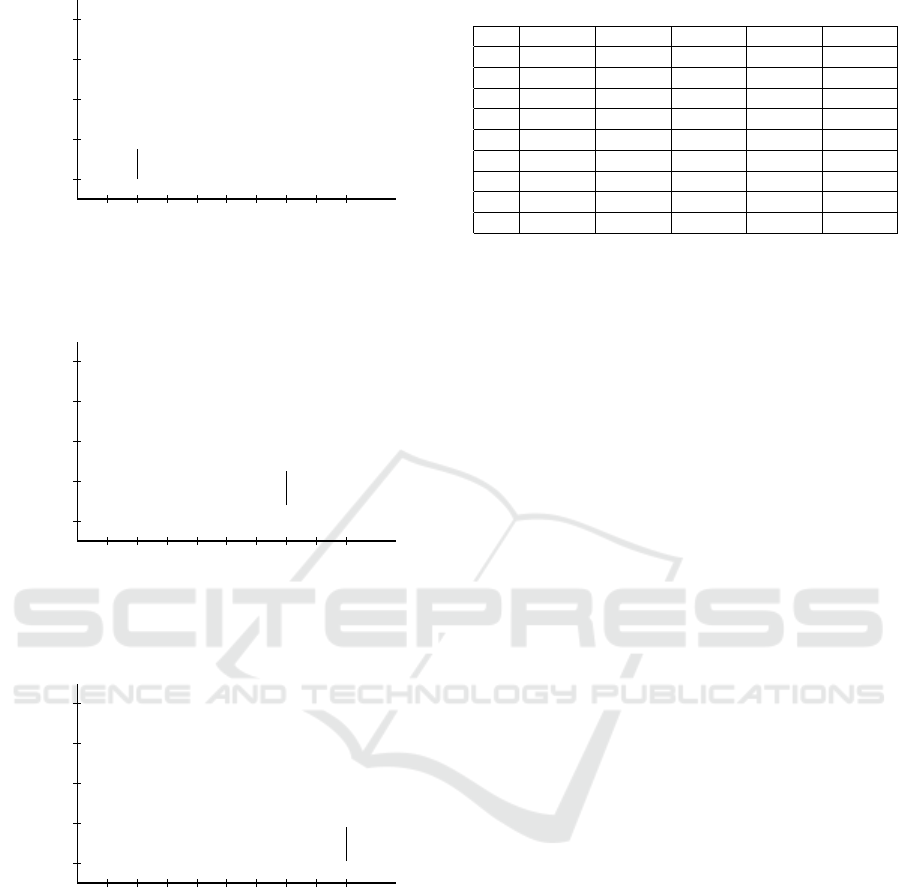
Figures 4, 5 and 6 describe the variable compo-

nents of the expected survival (

) of the differ-

ent strategies when q = 0.1, 0.4 and 0.7, respectively.

These examples illustrates two phenomena that holds

more generally. First, when q is low, any M

strategy

is less or equal to its companion Q

strategy. How-

ever, as q increases the M

strategies increase com-

pared to the Q

strategies and when q is sufﬁciently

high the M

strategies are equal or above their com-

panion Q

strategies.

Second, as q increases the optimal strategy shifts

to the higher (i.e., larger k) strategies. The intuition to

this is that when q is high then a sequential approach

has an advantage since it is more likely to eliminate

the system within a single or few period (compared to

the simultaneous that increases the probability of suc-

cess but at the cost of more time). In contrast, when

ICORES 2024 - 13th International Conference on Operations Research and Enterprise Systems

176

0 3 6 9

Var. component of exp. survival

Strategy

1.5

2.0

2.5

3.5

....

...

....

...

Optimum

Figure 4: The variable component of the expected survival,

and

, when N = 10, α = 0.5 and q = 0.1.

0 3 6 9

Var. component of exp. survival

Strategy

1.5

2.0

2.5

3.5

...

......

....

.....

....

.....

....

Optimum

Figure 5: The variable component of the expected survival,

and

, when N = 10, α = 0.5 and q = 0.4.

0 3 6 9

Var. component of exp. survival

Strategy

1.5

2.0

2.5

3.5

...

....

...

....

............................................. .............................................

r r r

Optimum

Figure 6: The variable component of the expected survival,

and

, when N = 10, α = 0.5 and q = 0.7.

q is low the advantage of saving time (since α < 1)

is relatively higher since it is more likely that multi-

ple tools will have to be used anyways due to the low

probability of each one to eliminate the system.

While the Q

strategies are lower than the M

strategies when q is sufﬁciently high, it appears that

this does not happen when it counts, i.e., the optimal

strategy is always less or equal to its companion

strategy. This can be gleaned from Table 1 that

describes the optimal strategy for different values of

Table 1: Optimal strategy for different values of α and q.

q α =0.1 α =0.3 α =0.5 α =0.7 α =0.9

0.1 Sim M

Seq

0.2 Sim M

Seq

0.3 M

Seq

0.4 M

Seq Seq

0.5 M

Seq Seq

0.6 M

Seq Seq Seq

0.7 M

Seq Seq Seq

0.8 M

Seq Seq Seq Seq

0.9 M

Seq Seq Seq Seq

Notes: Sim and Seq denote the purely simultaneous and

purely sequential strategies, respectively.

α and q (here, too, N = 10).

6 CONCLUSIONS

In this paper, we consider the question of whether

“putting all your eggs in one basket” is advisable or

not. This dilemma of pooling resources versus saving

assets for later needs is applicable to many ﬁelds of

operation. In our modelling, pooling resources does

not create an advantage or disadvantage in the prob-

ability of success, since we assume that the success

probability of each attack tool is identical and inde-

pendent. Instead, by pooling resources the hacker

trades off between waiting for the attack time to com-

plete before the success can be realized and the fact

that this attack time is shorter than a sequence of

single-tool attacks of the same number of tools.

Therefore, when the attack time of a multiple-tool

attack is very short, there is no advantage to the se-

quential approach and the optimal solution will be a

purely simultaneous attack. In contrast, if the attack

time is nearing the total time of a sequential attack,

then the optimal solution will be a purely sequential

attack. In between, we ﬁnd that the optimal solution

is mixed, where we show numerically that it is al-

ways preferable to begin with a simultaneous attack

and then complement it with a sequential attack. Ad-

ditionally, we demonstrate that as the probability of

success increases the optimum leans more towards a

sequential attack.

While our observations from the numerical exam-

ple are not formally proved, it appears the formu-

las that we derive for the M

and Q

strategies can

be mathematically analyzed to qualify these observa-

tions. It is also of interest to examine how changing

the modeling assumption that the probability of suc-

cess is independent of the other probabilities will af-

fect the results. This is left to future study.

Serial or Simultaneous? Possible Attack Strategies with an Arsenal of Attack Tools

177

REFERENCES

Andrad

ottir, S., Ayhan, H., and Down, D. G. (2017). Re-

source pooling in the presence of failures: Efﬁciency

versus risk. European Journal of Operational Re-

search, 256(1):230–241.

Cardoso, F., Costa, A., Norton, L., Senkus, E., Aapro, M.,

Andre, F., Barrios, C., Bergh, J., Biganzoli, L., Black-

well, K. L., et al. (2014). Eso-esmo 2nd interna-

tional consensus guidelines for advanced breast can-

cer (abc2). The Breast, 23(5):489–502.

Cui, P., Zhu, P., Xun, P., and Shao, C. (2018). Robustness of

cyber-physical systems against simultaneous, sequen-

tial and composite attack. Electronics, 7(9):196.

Dear, R. F., McGeechan, K., Jenkins, M. C., Barratt, A.,

Tattersall, M. H., and Wilcken, N. (2013). Combina-

tion versus sequential single agent chemotherapy for

metastatic breast cancer. Cochrane Database of Sys-

tematic Reviews, (12).

Lu, D.-Y., Wu, H.-Y., Yarla, N. S., Xu, B., Ding, J., and

Lu, T.-R. (2018). Haart in hiv/aids treatments: fu-

ture trends. Infectious Disorders-Drug Targets (For-

merly Current Drug Targets-Infectious Disorders),

18(1):15–22.

MacDonald, T. M., Williams, B., Webb, D. J., Morant,

S., Caulﬁeld, M., Cruickshank, J. K., Ford, I.,

Sever, P., Mackenzie, I. S., Padmanabhan, S., et al.

(2017). Combination therapy is superior to sequential

monotherapy for the initial treatment of hypertension:

a double-blind randomized controlled trial. Journal of

the American Heart Association, 6(11):e006986.

McNaughton, A. (2019). “parallel warfare” in conﬂicts with

limited political aims.

Phillips, A. N., Youle, M. S., Lampe, F., Johnson, M.,

Sabin, C. A., Lepri, A. C., and Loveday, C. (2003).

Theoretical rationale for the use of sequential single-

drug antiretroviral therapy for treatment of hiv infec-

tion. AIDS, 17(7):1009–1016.

Read, D., Antonides, G., Van den Ouden, L., and

Trienekens, H. (2001). Which is better: Simultane-

ous or sequential choice? Organizational Behavior

and Human Decision Processes, 84(1):54–70.

Sasikumar, K. (2019). India’s surgical strikes: Response to

strategic imperatives. The Round Table, 108(2):159–

174.

Soucy, R. (2018). Serial vs. parallel war: An airman’s view

of operational art. Technical Report ADA274440,

School of Advanced Military Studies, US Army Com-

mand and General Staff College, Leavenworth, KS.

Sunar, N., Tu, Y., and Ziya, S. (2021). Pooled vs. dedicated

queues when customers are delay-sensitive. Manage-

ment Science, 67(6):3785–3802.

Thompson, G. M. and Kwortnik Jr, R. J. (2008). Pooling

restaurant reservations to increase service efﬁciency.

Journal of Service Research, 10(4):335–346.

Xiong, G., Dong, X., Lu, H., and Shen, D. (2019). Re-

search progress of parallel control and management.

IEEE/CAA Journal of Automatica Sinica, 7(2):355–

367.

ICORES 2024 - 13th International Conference on Operations Research and Enterprise Systems

178