A Computer Vision Approach to Compute Bubble Flow of Offshore Wells

Rogerio C. Hart

and Aura Conci

Institute of Computing, Universidade Federal Fluminense, Niteroi, Rio de Janeiro, Brazil

Keywords:

Video Analysis, Segmentation, Flow Rate, Neural Network Model, Offshore Substructure.

Abstract:

This work presents two approaches for detecting and quantifying the offshore ﬂow of leaks, using video

recorded by a remote-operated vehicle (ROV) through underwater image analysis and considering the premise

of no bubble overlap. One is designed using only traditional digital image approaches, such as Mathematical

Morphology operators and Canny edge detection, and the second uses segmentation Convolutional Neural

Network. Implementation and experimentation details are presented, enabling comparison and reproduction.

The results are compared with videos acquired under controlled conditions and in an operational situation,

as well as with all previous possible works. Comparison considers the estimation of the average diameter of

rising bubbles, velocity of rise, leak ﬂow rate, computational automation, and ﬂexibility in bubble recognition.

The results of both techniques are almost the same depending on the video content in the analysis.

1 INTRODUCTION

Oil is one of the most important energy sources used

by man and of pollution to the environment. It is

composed of several elements, ranging from light

gas (methane) to heavy crude oil. Hydrocarbons are

formed by the grouping of atoms of carbon and hy-

drogen and can cause severe damage to the marine

environment. Oil pollution causes a collapse in vari-

ous activities carried out at sea, such as artisanal and

industrial ﬁshing, tourism, leisure, and navigation, in

addition to compromising conservation areas. The

sources of oil pollution at sea are diverse and gen-

erally come from transport by submarine pipelines.

The remotely operated underwater vehicles (ROVs)

are a safe alternative for inspections on offshore oil

drilling wells. These ROVs are equipped with cam-

eras capable of checking the infrastructure integrity

and leakage of transported materials (Capocci et al.,

2017). Monitoring and quantifying ﬂuid leaks is im-

portant to reduce environmental effects, (Kato et al.,

2017). Furthermore, quantifying the ﬂow rate un-

der the sea is required by environmental organiza-

tions that aim to inspect and regulate companies that

exploit such resources (Capocci et al., 2017; Kato

et al., 2017). Some approaches in the literature need

complex solutions that involve the utilization of ROVs

with acoustic sensors to identify and estimate the leak

https://orcid.org/0009-0003-0258-9410

https://orcid.org/0000-0003-0782-2501

ﬂow, where additional tools are required for complete

identiﬁcation (such as scanning the sub-seaﬂoor or

speciﬁc ROV positioning about the leak) making the

operation very difﬁcult and with great additional costs

(Nikolovska et al., 2008; R

omer et al., 2012; Sahling

et al., 2009). To periodically monitor, assess, and

inspect the wells and pipelines, many technologies

and methodologies have emerged, some using digital

image analysis (DIA) (Zielinski et al., 2010; Wang

et al., 2016). The use of DIA aims to perform a more

efﬁcient ﬂow estimation without the use of sophisti-

cated equipment or complex procedures for measure-

ments. The approach presented in this paper uses DIA

to compute bubble leak rate without extra equipment

attached to the ROV or complex operational proce-

dures to achieve results inside the acceptable amount

of variations (Ding, 2003).

Considering the related literature (see section 2)

the new contributions of this work are : (1) a method-

ology that uses DIA on ROV videos for estimation of

bubble ﬂow rate with acceptable processing time; (2)

a detailed algorithm able to efﬁciently estimate ﬂuid

ﬂow, equivalent diameter of a bubble, and bubble rise

speed and; (3) creation of a set of publicly available

videos that can be used as benchmarks (ground truths)

for future comparison by the interested community.

Section 2 discusses previous works related to the ap-

proach presented in Section 3 and 4. The results and

conclusions are presented subsequently in Sections 5

and 6 respectively.

664

Hart, R. and Conci, A.

A Computer Vision Approach to Compute Bubble Flow of Offshore Wells.

DOI: 10.5220/0012433500003660

Paper published under CC license (CC BY-NC-ND 4.0)

In Proceedings of the 19th International Joint Conference on Computer Vision, Imaging and Computer Graphics Theory and Applications (VISIGRAPP 2024) - Volume 3: VISAPP, pages

664-671

ISBN: 978-989-758-679-8; ISSN: 2184-4321

2 RELATED WORK

Boelmann and Zielinsk, in 2014, reported methods

and tools developed to characterize and measure gas

ﬂow on oil seeps. They used MATLAB to automat-

ically process videos pre-recorded by ROVs (Boel-

mann and Zielinski, 2014). In subsequent work, they

declare that one working day is needed to process

55,000 frames, showing that the approaches demand

a lot of time and computational effort (Boelmann and

Zielinski, 2015).

In order to characterize natural and anthropolog-

ical gas leaks from the seabed, Zelenka conducted a

3D analysis of the rising bubbles (Zelenka, 2014).

The author performs experiments using a glass box

and stereo-camera sensor. Automatic bubble detec-

tion and tracking algorithm based on the Kalman ﬁlter

is used for analysis. The work reports limitations of

using a single camera to estimate the velocity and size

of larger non-spherical bubbles (Zelenka, 2014). The

method proposed in the subsequent paper presents re-

liability and accuracy when used in places where there

is only one leak point, but unfeasible for situations

where multiple bubbles overlap (Jordt et al., 2015).

Vielst

adte et al. proposed a study on the impact of

methane emission at three abandoned drilling wells

located in the North Sea in Norway (Vielst

adte et al.,

2015). An ROV adapted with a funnel was used to

determine the ﬂow of emitted gas. Initially, the funnel

is used to determine the time it takes for the gas to ﬁll

the entire container. After, measurements of the size

versus quantity of the gas bubbles are analyzed using

the ImageJ software.

Wang and Socolofsky used MATLAB Image Pro-

cessing Toolbox to perform bubble counting, size

measurement, and quantiﬁcation of the ﬂow in a pre-

recorded video acquired by a ROV with a stereoscopic

imaging system in natural seaﬂoor leaks (Wang and

Socolofsky, 2015). Their algorithm identiﬁed and

quantiﬁed bubbles considering their clustering or

overlapping aspects using differentiation for thresh-

old. The validation of the system was proceeded

by laboratory experiments using plumes and their

method increased the accuracy of the size measure-

ment by 90%. In subsequent work (in 2016), the au-

thors improved their method by performing quantiﬁ-

cation of all bubbles in one frame per second to then

estimate ﬂow (Wang et al., 2016).

Al-Lashi et al., in 2016, conducted a study in the

North Atlantic on the size of bubbles under breaking

waves using a new instrument capable of recording

high-resolution video at 15 frames/s over a period of 8

hours (Al-Lashi et al., 2016), the authors described an

automatic algorithm capable of processing one frame

in 5 s and the Hough transform was used for bubble

analysis. However, It is not applicable in non-circular

or overlapping bubbles situations.

In 2020, Takimoto et al. combined image pro-

cessing and analysis techniques for segmenting bub-

bles (Takimoto et al., 2020) using records from a labo-

ratory and ultrasound acquisitions in order to compare

their results on underwater gas leaks. Bubble over-

lapping cases are handled by allowing proper volume

calculations (Honkanen et al., 2005). The errors were

less than 2% in rise speed, 10% in bubble rate, and

14% in leak rate.

In 2020, Li et al. employs a two-channel output

U-net model on images with overlapping bubbles to

generate a segmented particle image and a centroid

image of the particles. From these images, are used

the watershed approach to generate new segmented

and separated particles from the centroids (Li et al.,

2020).

In 2022 Hessenkemper et al. tested three differ-

ent methods based on Convolutional Neural Networks

(CNN’s) for segment bubbles and 2 methods to recon-

struct hidden overlapping parts (Hessenkemper et al.,

2022).

In the same year, Fernandes et al. compare several

methods for edge detection of leak bubbles in images

taken from ROV’s videos(Fernandes et al., 2022a).

A few months ago Hart et al. used a method based

on the Canny edge detection, on images taken from

underwater ROV videos, to identify and count leak

bubbles and compare the results with other methods

and human observation (Hart et al., 2023)

3 SEGMENTING BUBBLES

The underwater videos acquired by ROVs are in RGB

color, and the resolution and number of frames per

second are known a priori. The cv.videoCapture

function is used to separate video frames. It is not vi-

able to analyze that only one part of each frame, called

Region of Interest (ROI), is used. This part presents

all relevant information, and the limits of ROIs are ad-

justed manually for each video. In the reference (Hart

et al., 2023), it can be seen the images used in this

work.

Among possible neural network architectures, the

U-net was chosen because it is a network of interme-

diate complexity and presents very good results in a

range of segmentation applications. The name origi-

nates from the U-like shape of this CNN model. U-net

consists of an encoder and a decoder structure. The

ﬁrst reduces the width and height of an array but in-

creases the depth to extract features. The second does

A Computer Vision Approach to Compute Bubble Flow of Offshore Wells

665

the opposite in order to obtain local information from

the image. The encoder-decoder structures are cross-

connected (Ronneberger et al., 2015).

The Tensorﬂow and Keras libraries in Python lan-

guage were used for programming. The Google Co-

lab GPUs were used for training. The training im-

ages were taken from four videos. Two are captured

from experiments made in Universidade Federal Flu-

minense Fluid Mechanic laboratory considering air

bubbles propagating in water. The other two videos of

real leaks, with oil and gas bubbles in under sea deep

water. In all videos, original images were cropped to

256 X 256 pixels preserving the RGB color channels.

In total, 120 ROIs were used, taken from the real

leak video with oil bubbles, 46 from the real leak

video with gas bubbles, and 51 from the laboratory

video, totaling 217 images of 256 x 256 x 3 channels.

Of these, 163 were randomly chosen and reserved for

training and 54 for validation (a ratio of 75% for train-

ing and 25% for validation).

Due to the small number of images for training

and testing, it was necessary to use data augmenta-

tion, which consists of artiﬁcially increasing the train-

ing data by creating slightly modiﬁed copies of the

original dataset. For this, we use a library present in

the Keras package called IMAGEDATAGENERATOR.

The following arguments were used: rotation range =

90, width shift range = 0.3, height shift range = 0.3,

shear range = 0.5, zoom range = 0.3, horizontal ﬂip =

True, vertical ﬂip = True, ﬁll mode = ’reﬂect’).

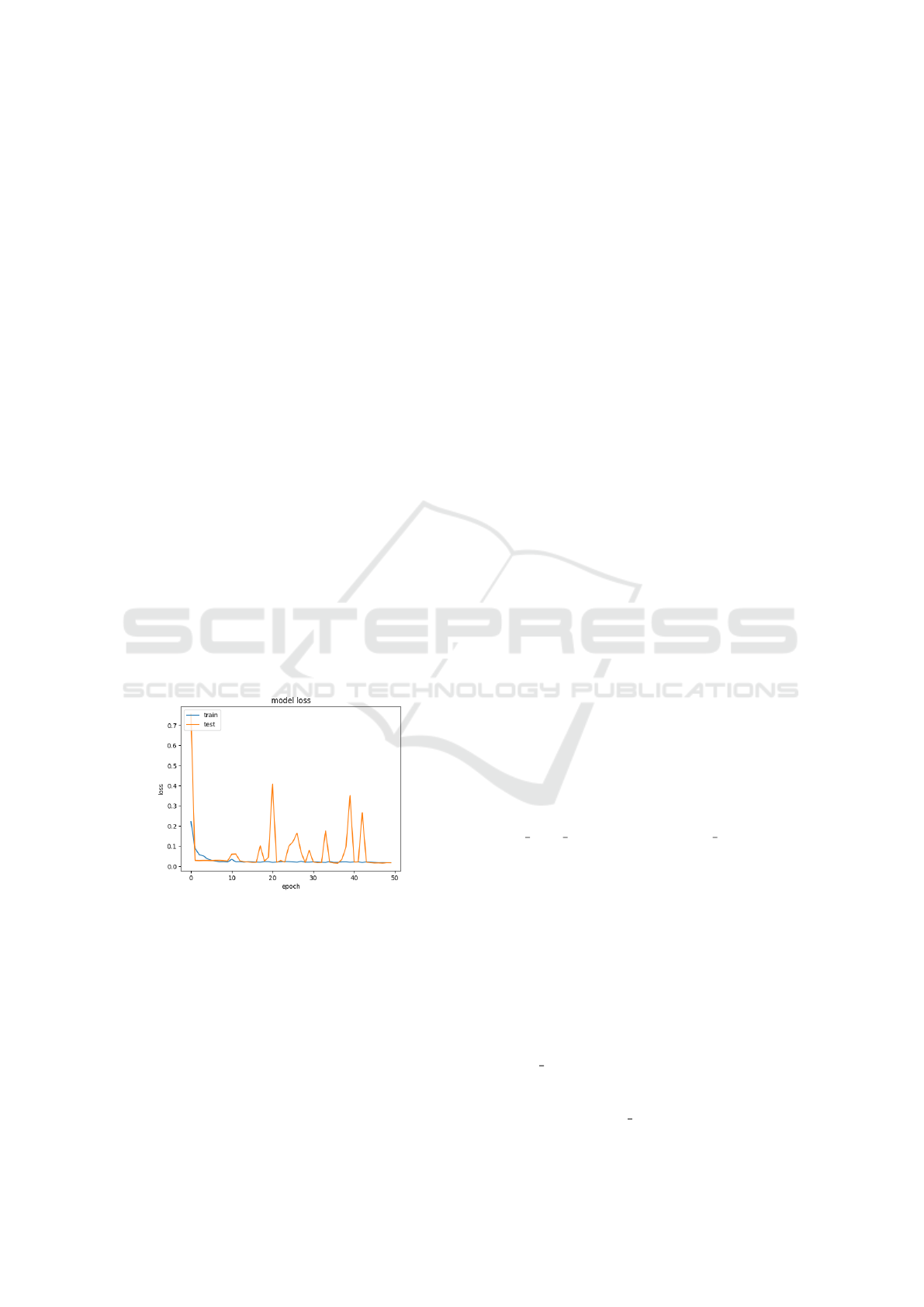
Figure 1: Learning curve for propose model, in the y-label

the loss in mean squared error and in the x-label the number

of epochs.

For training, the ADAM optimizer is used, with a

learning rate of 0.001. The regression loss function

used is the mean squared error and the accuracy is

used for evaluation of the results. The used steps per

epoch are 30, the same number for of steps are used

for validation, and up to 50 epochs are considered.

Fig. 1 presents the curves of training and testing the

model.

After validating, the net was used for the segment-

ing of the ROIs, i.e. bubbles were identiﬁed through

the network by using the ROIs frames for generating

masks with probabilities of the pixels present in the

image belonging to a bubble or not. ROI pixels with

a probability greater than or equal to 0.5 were consid-

ered as belonging to a bubble (positive) and smaller

as a background (negative).

3.1 Bubbles Segmentation by Image

Processing Methods

In this work two variations are used for the bubbles

recognition (we named them A and B). As Sections 5

and 6 will show, better results by using each one de-

pend on the expected or probable average distance

among bubbles and their distribution in the ROIs.

3.1.1 Variation A

This combination of traditional Image Processing

techniques has seven steps: (1) Conversion to gray

scale; (2) Histogram normalization; (3) Contrast ad-

justment; (4) Gradient computation; (5) Canny ﬁlter;

(6)Closing and; (7)Bubble full-ﬁll.

The steps (1), (2), (5), (6), and (7), were described

in detail in reference (Hart et al., 2023), and other

steps are described in the following lines. Fig. 2

presents the result of applying the steps described

above in one of the original images for example.

Contrast Adjustment.

To further increase the contrast between the bub-

bles and the background, the entire frame has been

adjusted by a simple sequence of multiplication and

inversion procedures.

First, the tones of the frame were inverted, by us-

ing:

New pix el intensity = 255 − pixel intensity. (1)

Then, the frame was multiplied by 1.5 (using

CV.MULTIPLY) in order to reinforce the dark tones.

Finally, the frame in process was inverted again (by

Equation (1) to increase now the lighter tones (by

multiplying them by 2). These values (1.5 and 2) are

chosen after several experiments.

Gradient Computation.

This step consists of taking the image resulting

from the previous step and applying the external gra-

dient operation in it. That is, it uses the MOR-

PHOLOGYEX OpenCV function with the parameter

MORPH

GRADIENT. In this process, the circular

4 × 4 structural element was used, it is obtained apply-

ing the function GETSTRUCTURINGELEMENT with

the parameter MORPH ELLIPSE .

VISAPP 2024 - 19th International Conference on Computer Vision Theory and Applications

666

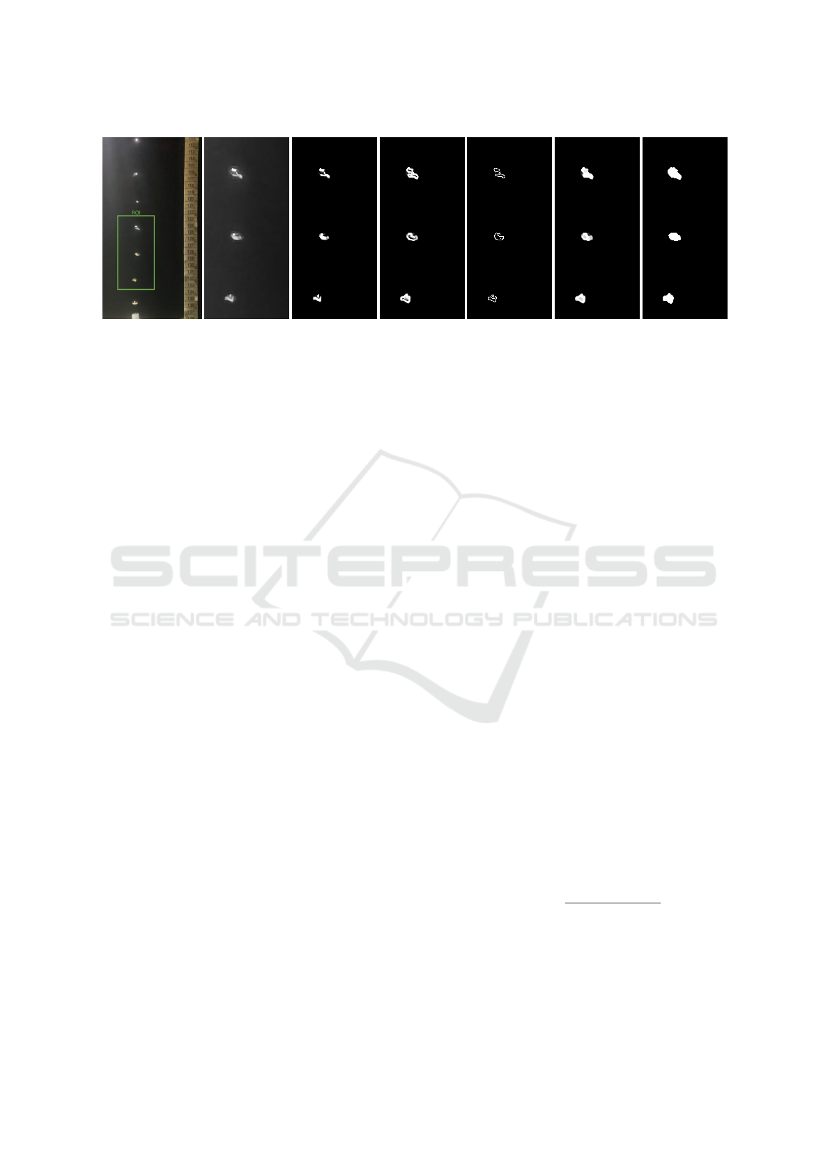
(a) RGB input and

its ROI.

(b) Y channel

conversion.

tion and contrast

adjusts.

(d) External

Morphological

Gradient.

(e) Canny Filter. (f) Closing. (g) Full-ﬁlled

bubble .

Figure 2: Outputs of each steps of the Variation A.

3.1.2 Variation B

Variation B has also seven steps. The ﬁrst ﬁve sets

(Conversion to gray-scale; Histogram normalization;

Contrast adjustment; Canny Filter and; Closing) and

the last step are the same of A, i. e. the same of the

previous variation. The different is the inclusion of

an Erosion and a Dilatation morphological operations

before the last step.During the tests, we realized, that

for small bubbles, the previous steps tended to detect

bubbles with areas larger than the real ones. To re-

duce the bubble area without losing shape, we used

the Erosion OPENCV function with a 3x3 rectangular

structural element followed by the Dilation operation

with a 2x2 rectangular structural element. We used

the functions CV.ERODE and CV.DILATE in these. .

3.1.3 Automatic Selection of Variations A or B

In the developed implementation, selection between

the variations A or B is made automatically. The de-

cision is based on the results of a process that apply

three simple steps: (1) Method A is applied to the

ﬁrst frame of the video to be analyzed; (2) The short-

est distance between the bubbles is computed in the

achieved results; (3) If this distance is greater than

the pre-deﬁned parameter, then variation A is used

throughout the video, otherwise, variation B is applied

to ir. The pre-deﬁned value was chose after some tests

and the value is 40 pixels.

For example, Fig2 presents well-spaced bubbles,

in which case method A will be applied. Fig. 3

presents some bubbles very close together, in which

case method B is chosen.

This test for variation selection must be used, dur-

ing experimentation, in some cases, variations A tends

to gather very close bubbles, but presents better re-

sults when there are bigger and more distant bubbles.

On the other hand, variation B presents better results

among closed and smallest bubbles.

4 BUBBLE FLOW EVALUATION

This section aims to present the used approach to

quantify the bubble’s average diameter, volume, and

rise speed. These elements are important to calcu-

late the leak ﬂow rate using image analysis of ROVs

recorded videos. In all the analysis we are consider-

ing the initial hypothesis of non-overlapping bubbles.

All analyzed techniques were implemented in Python,

using mainly functions already available in the Open

CV 4.7 library.

4.1 Average Diameter and Volume

Calculation

After the bubbles are identiﬁed in the frames and

are white-ﬁlled, the frames are processed by the

NUMPY. The NP.UNIQUE function counts the white

pixels present in each frame i. Then FINDCOUNTORS

function enumerates the separate bubbles in a frame i

) and provides an array with the position of bubble

edge pixels.

From the quantity of white pixels of each bubble,

we compute the total leak area (in mm) in the ROI of

the frame i using Equation (2):

total area =

total white pixels

resoltuion

(2)

Where resoltuion is the resolution of the video in

pixels/mm of frame i

From the total area, in mm, it is possible to cal-

culate the average diameter, D

avg

, of the bubbles in

the ROI of the frame i. For this, the bubble shape is

A Computer Vision Approach to Compute Bubble Flow of Offshore Wells

667

considered approximated by circles. That is, we use

the hypothesis that is possible to use Equation (3) for

diameter computation:

4 × total area

πn

(3)

where n

is number of bubbles presents in frame i

Considering that the bubble can be approximated

by spheres, using the average diameter, D

avg

, the av-

erage volume of one individual bubble in the frame i

, can be described by Equation (4):



avg



(4)

4.2 Average Rise Speed

The “geometric center” for each bubble in the ROI

can be approximated by its center of mass (CM).

These positions can be computed using the FIND-

CONTOURS function (that provides the contour pixels

of each bubble) and its center location is calculated by

using the edges pixels. The important data to be used

for bubble identiﬁcation (that must be saved) are the

perimeter and CM positions, that is the horizontal and

vertical position (x and y) of the CM for all bubbles in

a frame i. We also keep these data from the previous

frame i–1 for comparison.

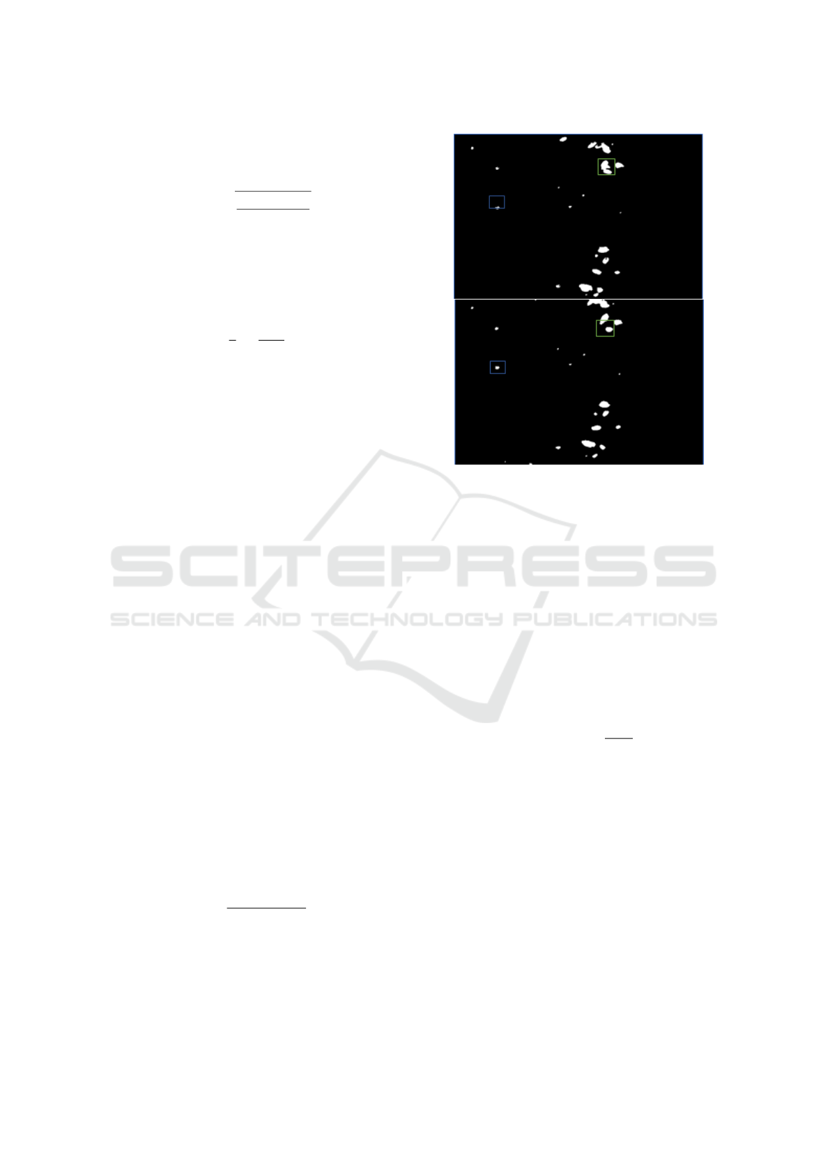
From this tree information, a bounding box is

drawn in an individual bubble in frame i–1, and the al-

gorithm will be looking for a bubble within the same

bounding box with a similar perimeter in the subse-

quent frame i. If in the frame there is at least one

bubble found, we calculate the distance between the

CM in frame i and frame i − 1. In cases where all bub-

bles have different perimeters or there are no bubbles,

we move on to the next bubble in the frame i–1, un-

til through over all the bubbles in the frame. Fig. 3

shows this process. This method neglects overlapping

bubbles that are identiﬁed as single bubbles like those

marked by the green box in Fig. 3.

The velocity for each bubble in the current frame

i can be calculated by the difference between the bub-

ble position in the current frame i and the previous

frame i − 1. As only the velocity in the vertical di-

rection is important, only this position is taken under

consideration for such a computation of v

cmi

− y

cm(i−1)

(5)

where y

cmi

is the vertical position of the CM bub-

ble in the frame i, and y

cm(i−1)

it position in previous

frame i − 1. The time interval t considered is the time

elapsed two consecutive frames that is the inverse of

the frames frequency, or the number of frames per

Figure 3: Naming the top image frame i − 1 and the bottom

one frame i. Bounding boxes show bubble search areas in

the next frame. If the bubble found has a perimeter close to

that of the previous frame (blue box) it is used for the calcu-

lation. In case of an overlapping bubble that is separated in

the subsequent frame or the shape is signiﬁcantly modiﬁed

(green box) it is disregarded.

second. The average velocity v

yMi

in frame i will be

the average of the velocities over all bubbles present

in the ROI for each frame i.

4.3 Average Bubble Flow Rate Q

From the equations of previous section, the average

ﬂow rate Q can calculated from Equation (6):

Q = n × V

ROI

(6)

where n is the number of bubbles presents in the ROI;

is the average volume of each bubble present in

the ROI; v

is the average rise speed of the bubble

in the video; H

ROI

is the height of the ROI, and the

average ﬂow in the video is Q. In the end all averages

were taken over all frames.

5 COMPARISONS

This section presents a comparison among results pre-

viously obtained experimentally, those estimated by

the previous approaches (Chagas, 2022)(Fernandes

et al., 2022b) and by actual implementation. The

aspects used to compare the results are the bubble’s

VISAPP 2024 - 19th International Conference on Computer Vision Theory and Applications

668

average diameter, rise speed, and ﬂow rate for each

video. All experimental and previous model results

are available (Chagas, 2022; Fernandes et al., 2022a).

To test the accuracy of the proposed algorithm, ex-

periments were performed using two types of videos:

videos acquired in controlled conditions in a labo-

ratory and real videos recorded under the sea. The

videos from laboratory named 021, 014, 022 and 024

are available at http://hidrouff.sites.uff.br/reconheci

mento-automatico-de-vazamento-em-estruturas-sub

marinas-raves, and the real videos with identiﬁcation

NA046-100 can be ﬁnd after permission (Wang et al.,

2016).

Previous implementations of our group use video

analysis to compute the volume and the rate of

ﬂow. One of these previous implementations uses

EMGUCV´s library and the following steps: (1)

Transform the image from RGB to Y channel; (2)

Apply a gradient ﬁlter using an elliptical 4×4 struc-

tural element; (3) Threshold the frames to a black and

white (binarization); (4) Apply morphological oper-

ations of opening and closing with elliptical struc-

turing elements of sizes 3×3 and 5×5, respectively

(Chagas, 2022). To obtain the bubbles ascend speed,

the EMGUCV´ S TRACKER functions were employed

by using the CHANNEL and SPATIAL RELIABILITY

TRACKING (CSRT) algorithm. However, it needs a

manual selection of a bounding box to track the mo-

tion of the select bubble (Chagas, 2022).

Videos 014, 021, 022, and 024 have 2400 frames

and a rate of 240 frames/s and 2.6 pixels/mm. For

these videos, the ROI used in this approach is the

region between the pixels [300:600] vertically and

[560:700] horizontally. The video NA046-100 has

1200 frames, with 30 frames/s and 4.15 pixels/mm,

the ROI considered for this is between the pixels

[400:800] vertically and [600:1200].

5.1 Comparing the Average Diameter

Table 1 presents results related to the average diam-

eter found experimentally in our lab (column EXP.),

by the (Chagas, 2022) (column Previous) and the two

approaches here presented (i.e. using Image Process-

ing (IP) and Neural Network (NN) approaches). Ana-

lyzing the Table, it can be seen that the current method

presented an average difference of only 3% from the

experimental results. This was 7% in the previous

implementation. The maximum difference between

the experimental and new approaches is 0.3mm while

comparing with the previous method shows 0.8mm.

Another advantage of the current implementation

is that there is no need for manual adjustments, in-

creasing the automation of the process. That is, the

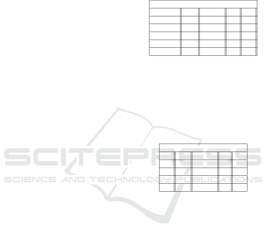
Table 1: Comparison for average diameter, in mm, of the

rising bubbles in videos, experimentally (EXP.), by previ-

ous and this work by using Image Processing (IP) and Neu-

ralNetwork(NN) approaches .

Average Diameter (mm)

ID Exp. Previous IP NN

014 5.3 5.7 5.4 5.1

021 7 7.5 6.9 6.9

022 7.5 8 7.5 7.5

024 8.2 9 8.1 8.1

Na046-100 2.9 2.8 3.2 3.2

approaches here presented improves the recognition

and estimation of bubble size.

5.2 Bubble Rise Speed Comparison

Table 2 presents results related to bubble rise veloc-

ity found experimentally in the lab, by the (Chagas,

2022) and here presented by approaches.

Table 2: Comparison for average Bubble rise speed in cm/s

in videos, experimentally, by previous and by here pre-

sented approaches.

Average rise speed (cm/s)

ID Exp Previous IP NN

014 33 34 37 36

021 31 30 31 31

022 33 32 33 33

024 38 37 38 36

Video Na046-100 does not show the average rise

speed in its results, for this reason, it does not appear

in Table 2. Regarding the rise speed estimation, both

here presented approaches show an average percent-

age difference of 3%.

The advance presented by the current method is

that while the previous one requires choosing a bub-

ble and manually tracing the bounding box, now it

becomes automatic. This manual selection can be a

problem in a video with many objects and various

rise speeds as in the video Na046-100. Moreover, the

current version allows automated measurement of the

rise speed of several bubbles simultaneously.

5.3 Comparing the Flow Rate

Estimation

Table 3 presents results related to ﬂow rate found ex-

perimentally in the lab, by the previous work [blind1]

and by this new approaches.

Regarding the ﬂow rate, the current method had

A Computer Vision Approach to Compute Bubble Flow of Offshore Wells

669

Table 3: Comparison for estimate ﬂow rate in mL/min in

videos, experimentally, by previous and here presented ap-

proaches.

Estimate Flow Rate Q in (mL/min)

ID Exp. Previous IP NN

014 96.6 97.2 109.1 92.5

021 86.6 86.9 85.1 83

022 131.9 133.5 135.3 134.8

024 234.9 229 232.6 225

Na046-100 30 33.2 31.1 30.3

a little worse difference in the experimental values,

with an average difference of 4% compared to the pre-

vious one of 3%.

Considering all the presented tables, for some

videos, the current method showed better results in

terms of diameter and rise speed but worse in terms

of ﬂow Q requiring further analysis in the future.

6 CONCLUSIONS

This paper presents new approaches to detect and

measure underwater leakage through video analysis.

The results are presented in terms of the diameter, vol-

ume, speed, and ﬂow rate of bubbles from leakages

carried out under controlled laboratory conditions or

in a real environment on the ocean ﬂoor. These are

useful for ﬂuid leak detection, calculating the leaked

oil volume, or other ROV imaging applications.

All steps of the proposed approach are presented,

allowing an easy reproduction since simple compu-

tational tools are used. Most of the videos used are

publicly available as indicated in Section 5, so the re-

sults can be compared by the interested community.

The current approaches show evolution in several

aspects compared to the previous. Such enhance-

ments are in (1) The estimation of the average di-

ameter; (2) The recognition and counting of bubbles,

and (3) The automation of the rise speed measure-

ment process with improvements in the results. An-

other important aspect is that the new implementation

is more ﬂexible, allowing the selection between two

Image Processing recognition or a Neural Network

based on the average distance of the bubbles in the

video.

The proposed implementation of the algorithm

shows potential for use in leak detection and estima-

tion. Furthermore, when compared with data from

ground truths, our approach presents good accuracy

and precision for important measurements such as

bubble diameter, volume, velocity, and ﬂow rate (in

a controlled environment and in videos of real situa-

tions reported in the literature).

However, we identiﬁed possible improvements of

the algorithm, including: (1)Treatment of overlap-

ping bubble; (2)Implementation of the automatic ad-

just of the ROI; (3) Flexibility in bubble detection for

different lighting and backgrounds; (4) Possibility of

bubble shrinkage throughout the water column (Wang

et al., 2020); (5) Diversions of bubble sizes and sub-

stances of the environment (Wu et al., 2021); (6) Al-

low ﬂuids in turbulent state (Wu et al., 2021); (7) Im-

plementation of artiﬁcial intelligence techniques for

calculation of the rise speed; (8) Test on a wider range

of videos with different lighting, backgrounds and

products.

We believe that with minimal modiﬁcations and

after the additional necessary validations, there is a

real possibility of the use of this approach in real situ-

ations, where the implementation is an embedded sys-

tem in the ROV.

ACKNOWLEDGEMENTS

Specially, the authors thank Professor Wang of the

University of Missouri for providing the actual videos

for comparing here (Wang and Socolofsky, 2015;

Wang et al., 2016; Wang et al., 2020). We ex-

press gratitude to the Hydrology Group of Universi-

dade Federal Fluminense for carrying out the labora-

tory experiments and permission to use their resulting

videos, We would like to thank A. F. Gonc¸alves and J.

V. de Souza Chagas for their guidance and assistance

during the project. A.C. acknowledge the support re-

ceived from CNPq, CAPES, and FAPERJ .

REFERENCES

Al-Lashi, R. S., Gunn, S. R., and Czerski, H. (2016). Auto-

mated processing of oceanic bubble images for mea-

suring bubble size distributions underneath breaking

waves. Journal of Atmospheric and Oceanic Technol-

ogy, 33(8):1701–1714.

Boelmann, J. and Zielinski, O. (2014). Characterization and

quantiﬁcation of hydrocarbon seeps by means of sub-

sea imaging. In 2014 Oceans-St. John’s, pages 1–6.

IEEE.

Boelmann, J. and Zielinski, O. (2015). Automated char-

acterization and quantiﬁcation of hydrocarbon seeps

based on frontal illuminated video observations. J.

Eur. Opt. Soc. Rapid Publ, 10.

Capocci, R., Dooly, G., Omerdi

c, E., Coleman, J., Newe,

T., and Toal, D. (2017). Inspection-class remotely op-

erated vehicles—a review. Journal of Marine Science

and Engineering, 5(1):13.

VISAPP 2024 - 19th International Conference on Computer Vision Theory and Applications

670

Chagas, J. V. d. S. (2022). Quantiﬁcation of underwater

bubble leaks applied to the oil industry (in portuguese:

Quantiﬁcac¸

ao de vazamentos de bolhas subaqu

aticas

aplicada

a ind

ustria de petr

oleo). M.Sc. Dissertation,

available in: http://www.ic.uff.br/index.php/pt/pos-

graduacao/teses-e-dissertacoes (2022).

Ding, Z. R. (2003). Hydromechanics. Higher Education

Press (Beijing).

Fernandes, A., Passos, F. G. O., and Conci, A. (2022a).

Comparing image preprocessing techniques for detec-

tion of bubbles in leaks. In 2022 29th International

Conference on Systems, Signals and Image Process-

ing (IWSSIP), volume CFP2255E-ART, pages 1–4.

Fernandes, A., Passos, F. G. O., and Conci, A. (2022b).

Comparing image preprocessing techniques for detec-

tion of bubbles in leaks. In 2022 29th International

Conference on Systems, Signals and Image Process-

ing (IWSSIP), volume CFP2255E-ART, pages 1–4.

Hart, R. C., Goncalves, L. M. G., Conci, A., and Ara-

gao, D. P. (2023). Comparing image processing tech-

niques for bubble separation and counting in under-

water leaks. In 2023 30th International Conference

on Systems, Signals and Image Processing (IWSSIP),

pages 1–5.

Hessenkemper, H., Starke, S., Atassi, Y., Ziegenhein, T.,

and Lucas, D. (2022). Bubble identiﬁcation from im-

ages with machine learning methods. International

Journal of Multiphase Flow, 155:104169.

Honkanen, M., Saarenrinne, P., Stoor, T., and Niinim

aki, J.

(2005). Recognition of highly overlapping ellipse-like

bubble images. Measurement Science and Technol-

ogy, 16(9):1760.

Jordt, A., Zelenka, C., Von Deimling, J. S., Koch, R.,

and K

oser, K. (2015). The bubble box: Towards

an automated visual sensor for 3d analysis and char-

acterization of marine gas release sites. Sensors,

15(12):30716–30735.

Kato, N., Choyekh, M., Dewantara, R., Senga, H., Chiba,

H., Kobayashi, E., Yoshie, M., Tanaka, T., and Short,

T. (2017). An autonomous underwater robot for track-

ing and monitoring of subsea plumes after oil spills

and gas leaks from seaﬂoor. Journal of Loss Preven-

tion in the Process Industries, 50:386–396.

Li, J., Shao, S., and Hong, J. (2020). Machine learn-

ing shadowgraph for particle size and shape char-

acterization. Measurement Science and Technology,

32(1):015406.

Nikolovska, A., Sahling, H., and Bohrmann, G. (2008).

Hydroacoustic methodology for detection, localiza-

tion, and quantiﬁcation of gas bubbles rising from the

seaﬂoor at gas seeps from the eastern black sea. Geo-

chemistry, Geophysics, Geosystems, 9(10).

omer, M., Sahling, H., Pape, T., Bohrmann, G., and Spieß,

V. (2012). Quantiﬁcation of gas bubble emissions

from submarine hydrocarbon seeps at the makran con-

tinental margin (offshore pakistan). Journal of Geo-

physical Research: Oceans, 117(C10).

Ronneberger, O., Fischer, P., and Brox, T. (2015). U-net:

Convolutional networks for biomedical image seg-

mentation.

Sahling, H., Bohrmann, G., Artemov, Y. G., Bahr, A.,

uning, M., Klapp, S. A., Klaucke, I., Kozlova, E.,

Nikolovska, A., Pape, T., et al. (2009). Vodyanit-

skii mud volcano, sorokin trough, black sea: Geolog-

ical characterization and quantiﬁcation of gas bubble

streams. Marine and Petroleum Geology, 26(9):1799–

1811.

Takimoto, R. Y., Matuda, M. Y., Oliveira, T. F., Adamowski,

J. C., Sato, A. K., Martins, T. C., and Tsuzuki, M. S.

(2020). Comparison of optical and ultrasonic meth-

ods for quantiﬁcation of underwater gas leaks. IFAC-

PapersOnLine, 53(2):16721–16726.

Vielst

adte, L., Karstens, J., Haeckel, M., Schmidt, M.,

Linke, P., Reimann, S., Liebetrau, V., McGinnis, D. F.,

and Wallmann, K. (2015). Quantiﬁcation of methane

emissions at abandoned gas wells in the central north

sea. Marine and Petroleum Geology, 68:848–860.

Wang, B., Jun, I., Socolofsky, S. A., DiMarco, S. F.,

and Kessler, J. (2020). Dynamics of gas bubbles

from a submarine hydrocarbon seep within the hy-

drate stability zone. Geophysical Research Letters,

47(18):e2020GL089256.

Wang, B. and Socolofsky, S. A. (2015). A deep-sea, high-

speed, stereoscopic imaging system for in situ mea-

surement of natural seep bubble and droplet charac-

teristics. Deep Sea Research Part I: Oceanographic

Research Papers, 104:134–148.

Wang, B., Socolofsky, S. A., Breier, J. A., and Seewald,

J. S. (2016). Observations of bubbles in natural seep

ﬂares at mc 118 and gc 600 using in situ quantitative

imaging. Journal of Geophysical Research: Oceans,

121(4):2203–2230.

Wu, H., Wang, B., DiMarco, S. F., and Tan, L. (2021). Im-

pact of bubble size on turbulent statistics in bubble

plumes in unstratiﬁed quiescent water. International

Journal of Multiphase Flow, -(-):103692.

Zelenka, C. (2014). Gas bubble shape measurement and

analysis. In German Conference on Pattern Recogni-

tion, pages 743–749. Springer.

Zielinski, O., Saworski, B., and Schulz, J. (2010). Marine

bubble detection using optical-ﬂow techniques. Jour-

nal of the European Optical Society-Rapid publica-

tions, 5.

A Computer Vision Approach to Compute Bubble Flow of Offshore Wells

671