Error Analysis of Aerial Image-Based Relative Object Position
Estimation
Zsombor P
´
ancsics
1,2 a
, Nelli Nyisztor
1,2 b
, Tekla T
´
oth
1 c
, Imre Benedek Juh
´
asz
2 d
,
Gergely Trepl
´
an
2
and Levente Hajder
1 e
1
Faculty of Informatics, E
¨
otv
¨
os Lor
´
and University Budapest, Hungary
2
Robert Bosch Kft. Budapest, Hungary
Keywords:
Aerial Imaging, Bird’s-Eye View, Error Analysis, Autonomous Navigation, Pose Estimation.
Abstract:
This paper presents a thorough analysis of precision and sensitivity in aerial image-based relative object posi-
tion estimation, exploring factors such as camera tilt, 3D projection error, marker misalignment, rotation and
calibration error. Our unique contribution lies in simulating complex 3D geometries at varying camera alti-
tudes (20-130 m). The simulator has a built-in unique mathematical model offering an extensive set of error
parameters to improve reliability of aerial image-based position estimation in practical applications.
1 INTRODUCTION
Over the last decade, the development of safer trans-
portation has become an important endeavour. New
requirements were imposed on manufacturers to im-
prove safety, increase comfort, and optimize energy
consumption. Therefore, the need for further traf-
fic analysis has increased, focusing on traffic partic-
ipants. However, using conventional methods like
radar- or LiDAR-based approaches, the analysis is an
expensive and time-consuming process.
Computer Graphics (CG) is often applied to sim-
ulate the urban environment for the testing of au-
tonomous vehicles. A popular open-source tool is
the CARLA simulator (Dosovitskiy et al., 2017) that
uses the Unreal Engine. Although CG-based tools
can generate specious pictures and videos, they do not
produce realistic recordings in many cases, especially
for range sensors like LiDAR or radar devices.
Traffic analysis, including relative object position
estimation, can be solved by a new aerial image-based
approach as well, which is a less expensive solution
since one downward looking camera is enough to
have a broad view of the traffic.
This paper collects and analyzes the different er-
a
https://orcid.org/0009-0002-9170-6908
b
https://orcid.org/0000-0002-6534-4715
c
https://orcid.org/0000-0002-7439-0473
d
https://orcid.org/0000-0002-6881-4604
e
https://orcid.org/0000-0001-9716-9176
ror factors of aerial image-based relative object posi-
tion estimation by simulating their effect on accuracy.
We determine the theoretical accuracy of this new ap-
proach and whether aerial imagery could replace or
complete the classical methods. Our results can foster
the development and validation of aerial image-based
relative object position estimation.
2 RELATED WORK
The task of object pose estimation in aerial imagery
has gained attention in recent years due to its wide
range of applications, i.e., autonomous navigation and
surveillance (Krajewski et al., 2018; Nguyen et al.,
2022; Nieuwenhuisen et al., 2016; Organisciak et al.,
2022; Patoliya et al., 2022). Thus, evaluating the lim-
itations, accuracy, and sensitivity of ADAS systems
is essential to ensure their effective and responsible
deployment in real-world scenarios.
Most pose estimation methods rely on a multi-
modal sensor input that provides 3D information of
the surroundings. (Kucharczyk et al., 2018) showed
that utilizing LiDAR point clouds, 2 and 8 cm
horizontal and vertical class-level accuracy can be
achieved while mapping a static environment. How-
ever, various scenarios require continuous localiza-
tion of dynamic objects over time. This can be re-
solved only by using data with high temporal granu-
larity. Apart from the data quality, high energy con-
656
Páncsics, Z., Nyisztor, N., Tóth, T., Juhász, I., Treplán, G. and Hajder, L.
Error Analysis of Aerial Image-Based Relative Object Position Estimation.
DOI: 10.5220/0012433300003660
Paper published under CC license (CC BY-NC-ND 4.0)
In Proceedings of the 19th International Joint Conference on Computer Vision, Imaging and Computer Graphics Theory and Applications (VISIGRAPP 2024) - Volume 3: VISAPP, pages
656-663
ISBN: 978-989-758-679-8; ISSN: 2184-4321
Proceedings Copyright © 2024 by SCITEPRESS – Science and Technology Publications, Lda.

sumption of 3D sensing devices cannot be neglected
either (Wang, 2021). In this paper, we present ac-
curacy analysis on aerial imagery, hence considering
only high-resolution, energy-efficient solutions.
While there are several works on the sensitiv-
ity and accuracy of image-based aerial pose esti-
mation, considering perspective mapping (Collins,
1992; Hartley and Zisserman, 2003), motion predic-
tion (Dille et al., 2011) and uncertainty in sensor po-
sition (Nuske et al., 2010). The work that served as a
solid reference for this report was written by (Babinec
and Apeltauer, 2016), who studied the errors caused
by the real world elevation, the positional inaccuracy
of the landmarks, and the distortion caused by the
camera.
Contributions. Beyond these factors, we analyze
the errors caused by the 3D geometry of the target
objects, possible camera tilts, and the uncertainty of
camera position. This allows a more realistic ap-
proach for dynamic scenarios. Finally, unlike other
works, we consider a wide range in altitudes (20-
130 m), enabling a much wider field of view and a
comprehensive comparison in projection errors.
3 OUR METHOD
This section outlines the basic virtual environment
and the working principles of the simulator.
First, we model a 3D environment: a traffic par-
ticipant and a marker (e.g. checkerboard) are defined
by their 3D model and 3D position. The camera is
modelled by its intrinsic and extrinsic parameters, see
Eqs. 1 - 4.
Second, the image capturing is modelled by a 2D
projection using a pinhole camera model. This step
projects the corner points of the original 3D object to
the 2D image plane, i.e. to pixel coordinates based
on the defined camera parameters (Figure 2). Also
considering camera distortion and/or camera tilt.
The third step is the simulation of the object de-
tection within the image, i.e., the determination of the
2D rotated bounding box, defined as the minimal-area
rectangle that covers the contour points of the object.
Finally, the simulator maps the objects back to the
original world coordinate system and compares their
original and new position. The Euclidean distance be-
tween their center points gives the error.
3.1 Initialization of 3D Environment –
Camera and Vehicle Models
In the initialization phase, the parameters and posi-
tions of the camera, the traffic participants and the
marker are defined as well as the the world scene to-
pography.
A general camera model is given by its intrinsic
and extrinsic parameters. The intrinsic parameters are
the focal length f
x
, f
y
and the principal point c
x
, c
y
,
which can be written in the form of the camera matrix.
K =


f
x
0 c
x
0 f
y
c
y
0 0 1


. (1)
The extrinsic parameters are represented by the 3D
rotation matrix R
c
and the 3D translation vector t
c
.
For the 3D-2D projection, a pinhole camera model is
used, described by the following equation:


u
v
1


= K

R
c
|t
c




x
y
z
1



, (2)
where [u v]
T
and [x y z]
T
are the pixel and spatial
coordinates, respectively. Radial and tangential dis-
tortions were also assumed which can be given with
five parameters. The related equations are as follows:
u
dist
= u(1 + κ
1
r
2
+ κ
2
r
4
+ κ
3
r
6
) +
2p
1
uv + p
2
(r
2
+ 2u
2
), (3)
v
dist
= v(1 + κ
1
r
2
+ κ
2
r
4
+ κ
3
r
6
) +
p
1
(r
2
+ 2v
2
) + 2p
2
uv, (4)
where r = ||u − c|| , u =

u v

T
, c =

c
x
c
y

T
, the
κ and p coefficients are the radial and tangential com-
ponents of the distortion model, respectively.
By default, the camera is looking downwards from
altitude h
c
in bird’s-eye view (Figure 3). If this is not
the case, and the camera has a tilt (pitch R
y
(β) or roll
R
x
(γ)), then the projection error will increase in most
of the cases due to the perspective view.
In the simulation, the virtual environment has a
flat surface, elevated topography was not modelled
yet.
The traffic participants are defined by their 3D
model and 3D position. Thus, cars are represented not
only by one rectangular cuboid, but by a more com-
plex car-like design - based on a commercial vehicle,
with different shapes on different z levels (Figure 1).
The lowest point of the vehicle, i.e. the wheel, should
always be on the ground. Therefore, its position can
be represented by 2D rotation R
o
and 2D translation
t
o
on the x-y plane. In this paper a single car is used
as traffic participant, but any object (pedestrian, two-
wheeler) can be used assuming an approximate 3D
model.
The ideal marker is a 2D planar object, which has
an altitude h
m
and a pattern definition. Ideally, its
Error Analysis of Aerial Image-Based Relative Object Position Estimation
657

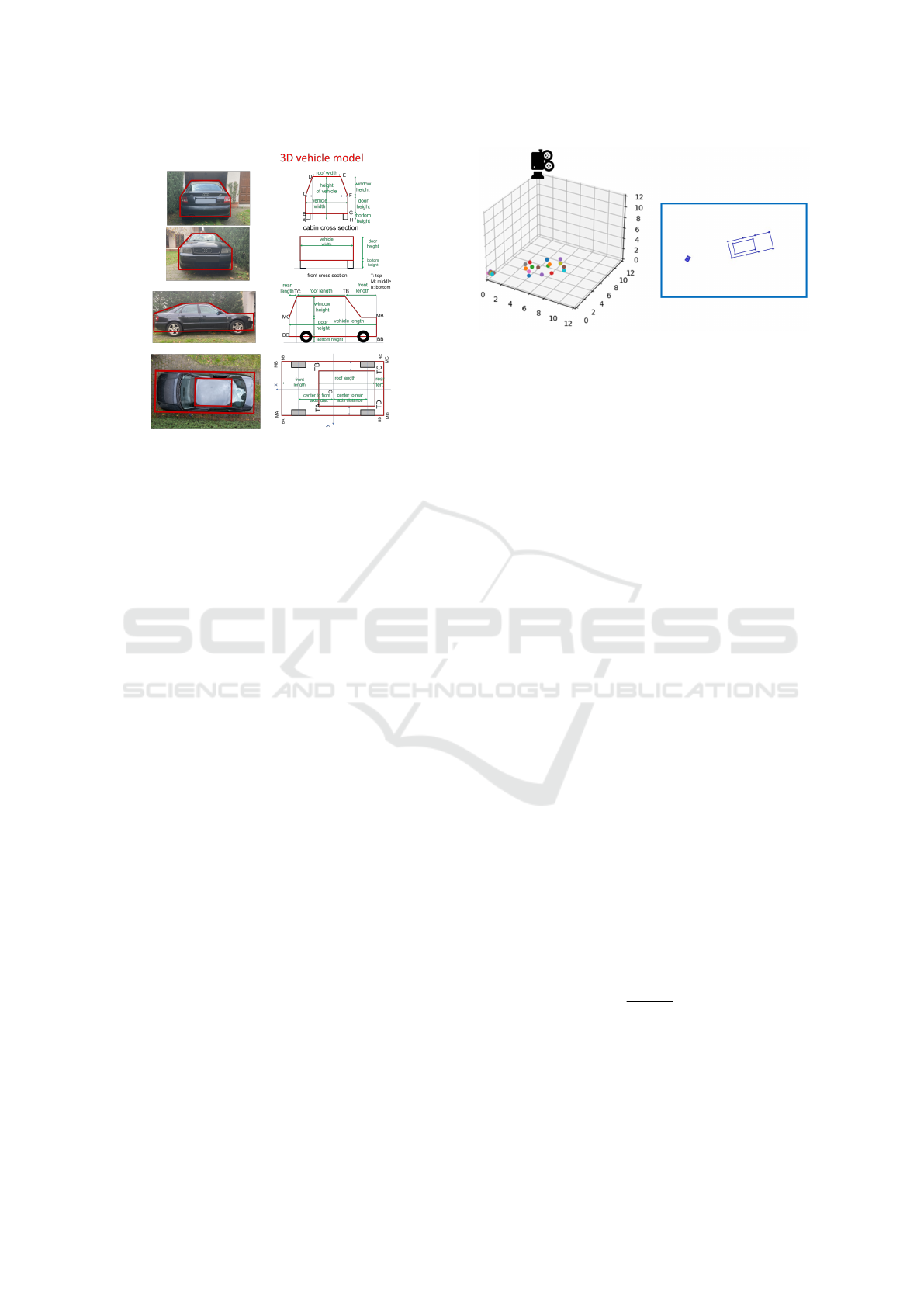
Figure 1: Abstract 3D representation of the vehicle.
center point should be placed in the origin, its edges
should be parallel with axes x and y, and its plane
should be perpendicular to axis z (Figure 6). Bias can
occur while installing the marker, so it can be tilted,
rotated and translated.
The rotation around axis z is called yaw and it can be
described by R
z
(α) (Eq. 5). Rotation biases around
axes y and x are called pitch R
y
(β) and roll R
x
(γ),
respectively (Eqs. 6 and 7).
R
z
(α) =


cos(α) −sin(α) 0
sin(α) cos(α) 0
0 0 1


(5)
R
y
(β) =


cos(β) 0 sin(β)
0 1 0
−sin(β) 0 cos(β)


(6)
R
x
(γ) =


1 0 0
0 cos(γ) −sin(γ)
0 sin(γ) cos(γ)


(7)
3.2 Simulator Working Principles,
Applied Camera and Vehicle Models
After the parameter initialization of the environment,
the image creation has to be simulated. This is done
by applying the central projection camera model, so
the simulator program projects the 3D metric coordi-
nates of the traffic participant onto the 2D image plane
pixel coordinates (Eqs. 2 - 4). The projection is visu-
alized in Figure 2. Its accuracy depends on the type
of the camera lens and its parameters.
After detection in the image, the objects can be
represented by minimum area rectangular boxes on
the image, also known as rotated bounding boxes.
This object representation is shown with a blue
Figure 2: Projection from the 3D world (left side) to the 2D
image plane (right side) using the central projection camera
model. Vehicle and marker feature points are visualized by
filled circles. Best viewed in color.
bounding box in Figure 4. It can be observed that
the original (red) and the projected (yellow) bounding
boxes does not completely coincide. This is caused by
the projection error, which is dependent on the cam-
era altitude, the distance between the traffic partici-
pant and the camera, the shape of the traffic partici-
pant (height and angularity), and the camera tilt.
Even though the traffic participant is represented
by a bounding box on the image plane, the position of
this box is unknown in the original ”real-world”, met-
ric coordinate system. Therefore it cannot be com-
pared to the original object position. The current and
the following paragraphs will explain the pixel to me-
ter conversion and the backmapping, based on the
marker pattern and position. It allows to determine
the position of the traffic participants in the original
coordinate system. To perform the pixel to meter con-
version, the pixel per meter ratio has to be calculated,
based on the original and projected marker pattern.
However this calculation is not enough in itself, be-
cause the marker could lay higher than the ground
level. In this case the pixel per meter ratio will define
only the ratio on the marker level, not on the ground
level, where the distance between the real and pro-
jected object (i.e., the error) is calculated. Section 3
highlights that the final error-distance measurement
is done on the ground level on z = 0 because during
the projection all object points were projected there.
Thus, the pixel per meter ratio needs to be adapted ac-
cordingly by the compensation of the pattern altitude.
This can be done by the following equation:
λ
z
=
h
c
− h
m
h
c
λ
m
, (8)
where λ
m
is the pixel per meter ratio on the marker
level, h
m
is the marker height, h
c
is the camera height,
and λ
z
is the pixel per meter ratio on the ground level.
Equation 8 is based on similar triangles as Figure 3
shows. The accuracy of the pixel per meter ratio cal-
VISAPP 2024 - 19th International Conference on Computer Vision Theory and Applications
658

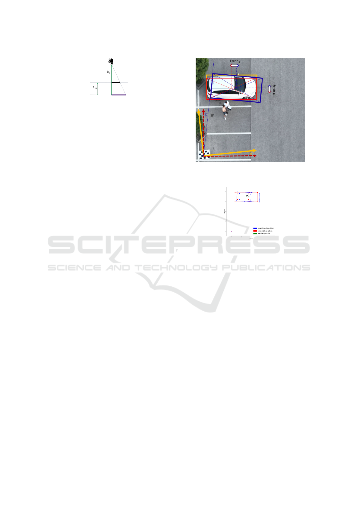
Figure 3: Adaptation of the pixel per meter ratio to the
ground level.
culation depends on the accuracy of the pattern recog-
nition, the marker altitude positioning, and marker
horizontality. Thus, uncertainty in any of these fac-
tors introduces pixel per meter ratio error, which in
turn results in center point distance error. The pixel
per meter ratio error λ
e
can be defined by the differ-
ence between the real λ
r
and calculated pixel per me-
ter ratio (λ
z
) (Eq. 9).
λ
e
= λ
z
− λ
r
, (9)
After the pixel per meter ratio on plane z = 0 is calcu-
lated (λ
z
), the coordinates of all object points can be
converted from pixels to meters (Eq. 10).

u
′
v
′

= λ
z

u
v

. (10)
The next step is backmapping, which will deter-
mine the position of the new bounding box in the
original coordinate system. It is important to note
that the detected marker position is not necessarily
in the origin of the picture, as it was in the original
coordinate system, because the camera is not neces-
sarily above the origin or because the marker could
be translated and rotated as well. The difference be-
tween the real and the detected marker positions de-
fine the backmapping transformation. This is shown
in the following equation:


u
′′
v
′′
w
′′


= −(R
mz
(α)R
my
(β)R
mx
(γ))


u
′
− m
cpx
v
′
− m
cpy
0


,
(11)
where m
cpx
and m
cpy
are the center point coordinates
of the detected marker and R
mz
(α)R
my
(β)R
mx
(γ) rep-
resents the initial rotation bias of the marker.
The backmapping is shown in Figure 4, where the
real-world coordinate system is marked with dashed
red arrows, with origin [0, 0, 0], and the red bounding
box represents the real position of the traffic partic-
ipant. Figure 4 demonstrates a setup where initially
a marker rotation bias occurred, demonstrated with
an orange α angle. This caused a rotation bias in
the position of the new (blue) bounding box during
backmapping (blue −α angle) on top of the already
existing projection error. The orange arrows represent
the coordinate system of the initially wrongly placed
Figure 4: Center points distance error caused by marker ro-
tation bias during backmapping.
Figure 5: Simulation of center points distance error caused
by projection error and marker-rotation bias.
marker, with α rotation bias compared to the correct
orientation, and the orange bounding box shows the
position of the projected traffic participant. Due to
the initial marker placement bias, a rotation error with
−α angle occurs on the orange bounding box, while it
is backmapped to the original coordinate system. The
result is the blue boundig box. The precision of the
backmapping depends on the precision of the initial
marker placement, as marker translation and rotation
bias can introduce an elementary error to the system.
Finally, the positions of the bounding boxes can
be compared and the difference can be calculated. It
is important to highlight that the comparison has to be
done on ground level, because all object points were
previously projected there and hereby lost their 3D
representation. The error is defined by the distance
between the center point of the the real and measured
bounding boxes as
Error =







u
v
0


−


u
′′
v
′′
0







2
. (12)
Figure 5 shows the visual output of the simulator
in a similar scenario as Figure 4, simulating a projec-
tion error and an initial marker rotation bias.
Error Analysis of Aerial Image-Based Relative Object Position Estimation
659

Figure 6: The visualization of error types.
The most important error factors influencing the
position estimation accuracy are collected in Sec-
tion 4. Their effects are analysed in Section 5 by using
the simulator program.
4 ERROR TYPES
There are two main considerations behind the
choices: (1) focus exclusively on factors relevant to
visual sensors, (2) maintaining a level of generality
that keeps our approach more widely usable within
the visual sensing domain. The studied error types
and their effect on position estimation accuracy are
pictured in Figure 6.
Uncertainty of the Marker Altitude. If there is
a difference between the real and the hypothetical
marker altitudes, where the altitude is measured from
the ground level, it leads to an error in the pixel per
meter adaption algorithm, which causes a biased pixel
per meter ratio, which finally causes the center point
distance error (unless the center point of the car is di-
rectly in the origin).
Marker positioning bias may occur during marker
installation and calibration. A wrongly calibrated
marker directly causes an error during the mapping
of the coordinate system, and results an elementary
center point distance error.
Non-parallel planes can be caused by a not directly
downward looking camera (non 90
◦
), by a steep scene
topography, by a tilted marker installation, or by the
combinations of these factors. This paper focuses
on the simulation of camera and marker tilt, which
causes the same error as a plane with a slope.
Unknown 3D Structure of the Projected Objects.
Traffic participants are modelled in 3D (Figure 1),
causing a projection error. In the absence of a precise
model, this error cannot be compensated, thus lead-
ing to misalignment (Figure 4 red - orange boxes).
This error increases with larger perspective angle, i.e.,
Table 1: Experiment parameters.
Parameter x/γ y/β z/α
Camera pos. 0-50 m 0-50 m 0-130 m
Camera tilt 0-180
◦
0-180
◦
0-180
◦
Object pos. 0-50 m 0-50 m —
Marker pos. bias 0-1 cm 0-1 cm 0-1.5 cm
Marker rot. bias 0-3
◦
0-3
◦
0-3
◦
when the object is at the edge of the image, or when
its height relative to the camera altitude is larger.
Camera distortion depends on the camera lens type
and quality. It leads to wrong pixel per meter ratio and
to distorted object outlines, especially on the edge of
the image. It can be compensated by camera calibra-
tion methods.
5 EXPERIMENTAL RESULTS
In this section, the previously collected error types are
simulated and their effects on the position estimation
accuracy are visualized and evaluated.
The error of accuracy is measured in two ways,
applying the pixel per meter error (Eq. 9) and the dis-
tance of the original and back-projected-back-mapped
traffic participant center points (Eq. 12), where the
center point is defined in a way that it means the cen-
ter point of the minimum area rectangle around the
traffic participant outermost corner points.
The experimental parameters and ranges are sum-
marized in Table 1.
5.1 Error due to the Uncertainty of the
Marker Altitude
In this section, the center points distance error and
the error of pixel per meter ratio are simulated and
analysed, caused by the marker-altitude uncertainty.
All other error factors are zero.
Marker Below the Camera. The marker altitude un-
certainty causes a linear pixel per meter ratio error,
but does not cause any center point differences er-
rors. Even tough the outline increases, it increases
centrally, therefore the center point remains in posi-
tion.
Marker Not below Camera. In the next setup, we
fixed the marker altitude uncertainty to 0.06 m. The
camera and the traffic participants are moving to-
gether along axis x. Thus, no projection error occurs.
In this case, the constant marker-altitude uncertainty
causes constant pixel per meter ratio error, regardless
of the distance between the marker and the camera.
However, the center points difference error increases
linearly as the camera distance increases.
VISAPP 2024 - 19th International Conference on Computer Vision Theory and Applications
660

5.2 Error due to Marker Positioning
In this section we analyse the center points distance
error and the pixel per meter ratios error, caused by
the marker positioning biases, while keeping other er-
ror factors zero.
5.2.1 Marker Translation Bias
Three different marker translation biases were stud-
ied. Based on the simulator results, translation ap-
plied to the marker separately or combined into direc-
tions x and y does not affect the pixel per meter ratio.
However, increasing its distance from the center point
causes a linear growth in the error.
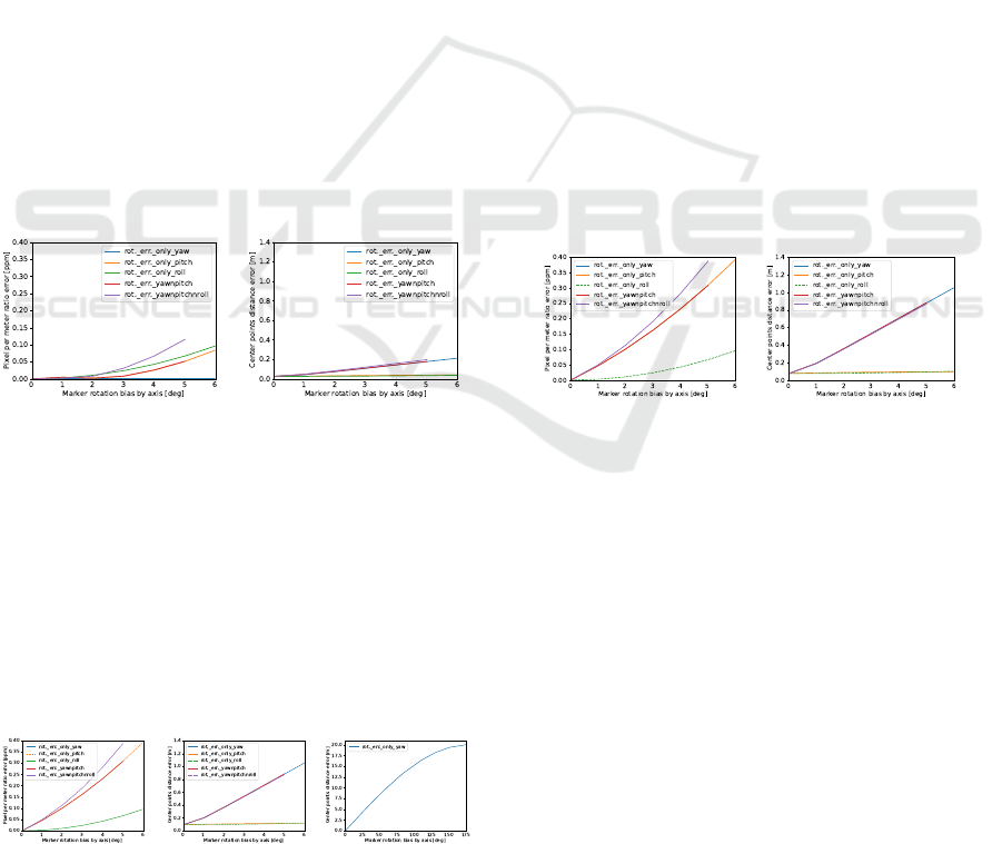
5.2.2 Marker Rotation Bias
Five different marker-rotation biases are simulated.
They are visualized with different graph colors, yaw -
blue, pitch - orange, roll - green, yaw and pitch at the
same time - red, yaw and pitch and roll at the same
time - purple.
Close to Camera. The following figures show the
simulation of errors caused by marker-rotation bias,
where the marker is laying in position [0, 0, 0.2] but
the camera and the vehicle position is not above the
origin, but in [2, 0].
(a) ppm. ratio error (b) cp. dist. error
Figure 7: Pixel per meter ratio error (a), center points dis-
tance error (b) caused by marker rotation bias, close to cam.
Figure 7a highlights the pixel per meter ratio er-
ror w.r.t marker-rotation biases around the x; y; z; xy;
xyz axes. Whereas Figure 7b shows the center point
differences w.r.t. same rotation biases.
Far from Camera. Figure 8 shows the errors caused
by marker-rotation biases, where the marker is origi-
nally laying in position [0, 0, 0.2], while the camera
and the vehicle position is not in origin, but in [10, 0].
(a) ppm. ratio error (b) cp. dist. error (c) cp. dist. error
Figure 8: Pixel per meter ratio error (a) and center points
distance error (b,c) caused by marker rotation biases.
Figure 8a shows the pixel per meter ratio error ten-
dency depending on the marker-rotation around the
x; y; z; xy; xyz axes. Figure 8b shows the center
point differences tendency regarding the same rota-
tions. Figures 8a and 8b show that the most signifi-
cant error is caused by the rotation bias around z axis
(yaw). Figure 8c shows the center points distance er-
ror tendency in a wider rotation angle range.
Two conclusions can be drawn from Figures 7 and
8. First, the center points distance error increases
when the marker-rotation bias increases. Second, this
error is even greater when increasing the distance be-
tween the vehicle and the origin. At a distance of 30
m from camera, even a one-degree marker yaw devi-
ation adds another 31 cm error. This happens because
the distant objects move on a longer arc.
5.2.3 Marker Rotation Bias with Fixed
Translation
The following section shows the simulation of er-
rors caused by marker-rotation bias with fixed 0.02
m marker translation bias along axis x.
The marker is laying in position [0.02, 0, 0.2] and
the marker rotation biases around axes x; y; z; xy; xyz
are swept, the camera position is in [10, 0, 100], the
vehicle is directly below the camera. All of the other
error factors are zero.
(a) ppm. ratio error (b) cp. dist. error
Figure 9: Pixel per meter ratio error (left) and center points
distance error (right) caused by marker rotation bias by axis
with a fixed marker translation bias, far from the camera.
Figure 9 shows similar behavior as Figure 7. It
is important to note that the most significant error is
caused by rotation, not by the translation bias, which
has a large effect on accuracy of distant objects.
5.3 Error due to Non-Parallel Planes
In this section the errors caused by non-parallel planes
will be presented that occurs due to different tilts.
Marker Tilt. Marker pitch and roll tilts cause non-
parallel plane problem. These errors are already sim-
ulated in Section 5.2.2.
Camera Tilt. The experiments include camera tilt on
the roll, pitch and yaw axes. Figure 11 shows that
Error Analysis of Aerial Image-Based Relative Object Position Estimation
661

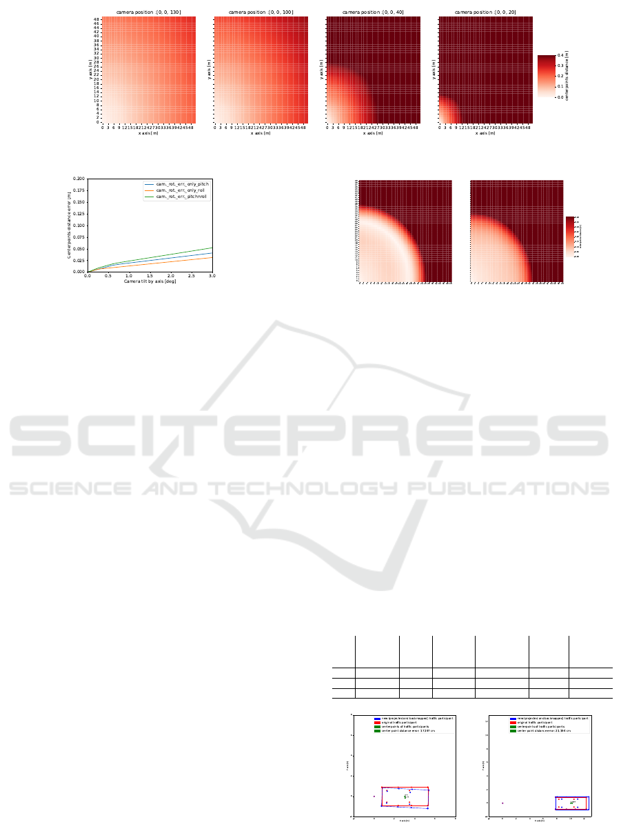
Figure 10: Center points distance error caused by the 3D-2D perspective projection, from different camera altitudes.
Figure 11: Center points distance error caused by different
camera tilts, directly above the marker.
the final center points distance error increases with
increasing angle values.
5.4 Error due to Unknown 3D Structure
In this section the bounding box center points dis-
tances are analysed, depending on the vehicle position
and camera (lowered) altitude.
Since the traffic participants are modelled in 3D,
see in Figure 1, it affects their position estimation
from perspective view (because of projection error).
In the absence of a precise 3D model, this error can-
not be compensated by back-projection and leads to
bounding box misalignment. In order to demonstrate
it, the vehicle is moved around the scene with fixed
camera position above the origin. By applying a lower
camera altitude, the perspective view increases, lead-
ing to a growth for projection and center point differ-
ence error. This is showed on Figure 10 with camera
altitudes of 130 m, 90 m, 40 m and 20 m.
5.5 Error due to Camera Distortion
Two types of camera distortion are analyzed in this
section, that are barrel and pincushion distortions.
They occur by non calibrated cameras, depending on
the camera lens type and quality.
Figure 12 shows the applied camera distortions in
the simulator. Note its comparison with the second
plot in Figure 10, where no distortion was applied.
They have the same scaled color bars and they are
simulating the same scenario from 100 m altitude. It
can be concluded that the camera distortions increase
Figure 12: Center points distance error due to barrel (left)
and pincushion (right) camera distortions across the scene.
the error, especially on the edges, highlighting the im-
portance of the proper calibration of the camera.
5.6 Complex Scenarios
In this section, the bounding boxes center points dis-
tance error are simulated in real, complex scenarios,
defined by the parameters listed in Table 1.
Several scenarios are covered in order to form the
final conclusions. Three scenarios are highlighted in
Table 2 which demonstrates: (a) the robustness of the
system in close camera range with huge biases (visu-
alised in Figure 13a), (b) perspective distortion from
low camera altitude (visualised in Figure 13b), (c)
close camera range, with realistic biases.
Table 2: Complex scenarios parameters.
cam. veh. cam. marker marker cp.
no. pos. pos. rot. transl. bias rot. bias distortion
[x, y, z] [x,y] [α,β,γ] [x,y,z] 10
−2
[α,β,γ] error
a) [0, 0, 100] [3, 0] [0, 0.7, 0] [1, 1, 1.5] [3, 0, 0] 17.2 cm
b) [0, 0, 30] [10, 0] [0, 0, 0] [0, 0, 0] [0, 0, 0] 21.19 cm
c) [0, 0, 100] [3, 0] [0, 0.7, 0] [1, 0, 0] [1, 1, 0] 4.82 cm
(a) (b)
Figure 13: Center point distance error in complex scenarios.
VISAPP 2024 - 19th International Conference on Computer Vision Theory and Applications
662

6 CONCLUSION AND FUTURE
WORK
Through a systematic experimental setup, covering
diverse scenarios, we identified key factors influenc-
ing the accuracy of aerial image-based relative object
position estimation, including plane misalignment,
3D structure uncertainties and calibration errors. We
developed mathematical models, and used them in a
unique simulator that allowed us to conclude the fol-
lowings.
Our main contribution is the evaluated projection
error of 3D-modelled traffic participants. We showed
that the distortion originating from this factor is min-
imal, when the object is below the camera (nadir) and
increases as the object moves away from the camera.
We also demonstrated that, the initial angular mis-
alignment of the marker and camera causes a signif-
icant error. Thus, a precise calibration is crucial for
aerial image-based positioning, especially for long-
range applications.
Setting the distortion and bias parameters to val-
ues that correspond to practically relevant use cases,
we found that in near range, the error of aerial image-
based relative object position estimation is less than
10 cm. Thus, under the aforementioned circum-
stances, the novel approach can achieve a precision
comparable to other, more complex, radar or LiDAR-
based methods. To reach a better precision, or a sim-
ilar precision for a wider range, one can use, for in-
stance, complex camera systems.
Future Work. In this stage, the simulator is ready
to build up a simple 3D world-model and simulate
basic error factors. Further developments can lead
to a more realistic simulated environment, including
topography; different weather conditions (rain/fog);
random noise. More realistic camera models can be
implemented, considering resolution, field of view,
and gimbal stabilization biases. Finally, more so-
phisticated error metrics can be developed for further
analysis.
ACKNOWLEDGEMENTS
Project no. C2286690 has been implemented with the
support provided by the ministry of culture and in-
novation of Hungary from the national research, de-
velopment and innovation found, financed under the
KDP-2023.
Furthermore, I would like to express my gratitude
to M
´
at
´
e Fugerth, Marcell Nagy, Anna V
´
amos and to
my company Robert Bosch Kft. for supporting my
project.
REFERENCES
Babinec, A. and Apeltauer, J. (2016). On accuracy of posi-
tion estimation from aerial imagery captured by low-
flying uavs. International Journal of Transportation
Science and Technology, 5(3):152–166. Unmanned
Aerial Vehicles and Remote Sensing.
Collins, R. T. (1992). Projective reconstruction of approxi-
mately planar scenes. volume 1838, page 174 – 185.
Dille, M., Grocholsky, B., and Nuske, S. (2011). Per-
sistent visual tracking and accurate geo-location of
moving ground targets by small air vehicles. In In-
fotech@Aerospace 2011, Reston, Virigina. American
Institute of Aeronautics and Astronautics.
Dosovitskiy, A., Ros, G., Codevilla, F., L
´
opez, A. M., and
Koltun, V. (2017). CARLA: an open urban driving
simulator. In 1st Annual Conference on Robot Learn-
ing, CoRL 2017, Mountain View, California, USA,
November 13-15, 2017, Proceedings, volume 78 of
Proceedings of Machine Learning Research, pages 1–
16.
Hartley, R. and Zisserman, A. (2003). Multiple View Geom-
etry in Computer Vision. Cambridge University Press,
New York, NY, USA, 2 edition.
Krajewski, R., Bock, J., Kloeker, L., and Eckstein, L.
(2018). The highd dataset: A drone dataset of natural-
istic vehicle trajectories on german highways for val-
idation of highly automated driving systems. In 2018
21st International Conference on Intelligent Trans-
portation Systems (ITSC), pages 2118–2125.
Kucharczyk, M., Hugenholtz, C. H., and Zou, X. (2018).
Uav–lidar accuracy in vegetated terrain. Journal of
Unmanned Vehicle Systems, 6(4):212–234.
Nguyen, K., Fookes, C., Sridharan, S., Tian, Y., Liu, F., Liu,
X., and Ross, A. (2022). The state of aerial surveil-
lance: A survey. arXiv preprint arXiv:2201.03080.
Nieuwenhuisen, M., Droeschel, D., Beul, M., and Behnke,
S. (2016). Autonomous navigation for micro aerial
vehicles in complex GNSS-denied environments. J.
Intell. Robot. Syst., 84(1-4):199–216.
Nuske, S. T., Dille, M., Grocholsky, B., and Singh, S.
(2010). Representing substantial heading uncertainty
for accurate geolocation by small UAVs. In AIAA
Guidance, Navigation, and Control Conference, Re-
ston, Virigina. American Institute of Aeronautics and
Astronautics.
Organisciak, D., Poyser, M., Alsehaim, A., Hu, S., Isaac-
Medina, B., Breckon, T., and Shum, H. (2022). UAV-
ReID: A benchmark on unmanned aerial vehicle re-
identification in video imagery. In Proceedings of the
17th International Joint Conference on Computer Vi-
sion, Imaging and Computer Graphics Theory and
Applications. SCITEPRESS - Science and Technol-
ogy Publications.
Patoliya, J., Mewada, H., Hassaballah, M., Khan, M. A.,
and Kadry, S. (2022). A robust autonomous naviga-
tion and mapping system based on GPS and LiDAR
data for unconstraint environment. Earth Sci. Inform.,
15(4):2703–2715.
Wang, P. (2021). Research on comparison of LiDAR and
camera in autonomous driving. J. Phys. Conf. Ser.,
2093(1):012032.
Error Analysis of Aerial Image-Based Relative Object Position Estimation
663