Automated Palette Cycling Animations

Ali Sattari Javid

and David Mould

School of Computer Science, Carleton University, Ottawa, Canada

Keywords:

Animation, Image Processing, Palette Cycling, Pixel Art.

Abstract:

We propose an automated method for palette cycling, a technique for animation storage and playback. A

palette cycling animation uses a ﬁxed map of indices over the entire animation; each frame, the color lookup

table accesses by the indices changes. Historically, palette cycling animations were created manually. Here,

we present a method that automatically creates a set of palettes and an index map from an input video. We use

optimization, alternating between phases of choosing per-frame palettes and determining an index map given a

ﬁxed set of palettes. Our method is highly effective for scenarios such as time-lapse video, where the lighting

changes dramatically but there is little overall motion. We show that it can also produce plausible outcomes

for videos containing large-scale motion and moving backgrounds; palette rotations with these features are

especially difﬁcult to craft by hand. We demonstrate results over a variety of input videos with different levels

of complexity, motion, and subject matter.

1 INTRODUCTION

This paper describes an automated system for con-

verting a video into an animation using palette cy-

cling. Palette cycling is a technique for saving mem-

ory by using a shared set of palette indices across all

frames, only varying the per-frame palette. Note that

this is the opposite of a more conventional compres-

sion scheme such as that used for animated GIFs, in

which the palette is shared and the per-frame pixel

indices differ. Thus, in palette cycling, a different

palette index is needed for any two pixels which dif-

fer at any frame in the animation: the animation over

all frames and the color structure of individual frames

are jointly encoded into a single index map. Despite

this severe restriction, it is possible to encode seem-

ingly complex animations into small palettes. A hand-

crafted palette cycling animation by artist Mark Fer-

rari is shown in Figures 1 and 2, giving a sense of

what is possible; Figure 1 shows the palettes and in-

dex map, and Figure 2 shows examples of individual

frames.

Handcrafted palette cycling was a common tech-

nique for representing animations in the early days

of home computers, and can be used today when-

ever memory restrictions are severe. Palette cycling

typically produces much smaller ﬁles than the more

https://orcid.org/0009-0003-0217-782X

https://orcid.org/0000-0001-5779-484X

common encoding of per-frame index into a common

palette, but comes with signiﬁcant limitations in re-

producing dynamic content.

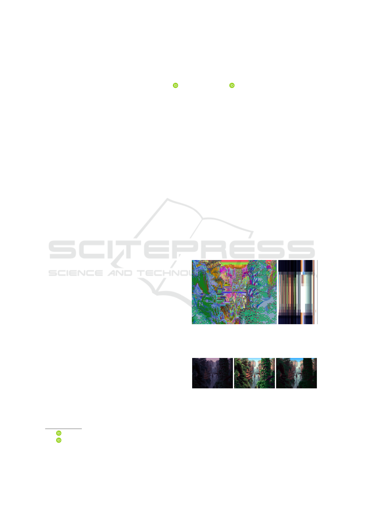
Figure 1: Visualization of index map (left) and palettes

(right) for an animation created by hand by Mark Ferrari.

Each palette is one horizontal strip, with the time sequence

progressing top to bottom.

Figure 2: Using a ﬁxed index map, Ferrari created different

times of day just by changing the palette colors.

Handcrafted palette cycling animations typically

used ﬁxed views and contained little motion. Small,

repetitive motions were possible, such as snow falling

or waves crashing on a beach. Large-scale color

changes, due to night falling or a change in season,

Javid, A. and Mould, D.

Automated Palette Cycling Animations.

DOI: 10.5220/0012432500003660

Paper published under CC license (CC BY-NC-ND 4.0)

In Proceedings of the 19th International Joint Conference on Computer Vision, Imaging and Computer Graphics Theory and Applications (VISIGRAPP 2024) - Volume 1: GRAPP, HUCAPP

and IVAPP, pages 115-126

ISBN: 978-989-758-679-8; ISSN: 2184-4321

115

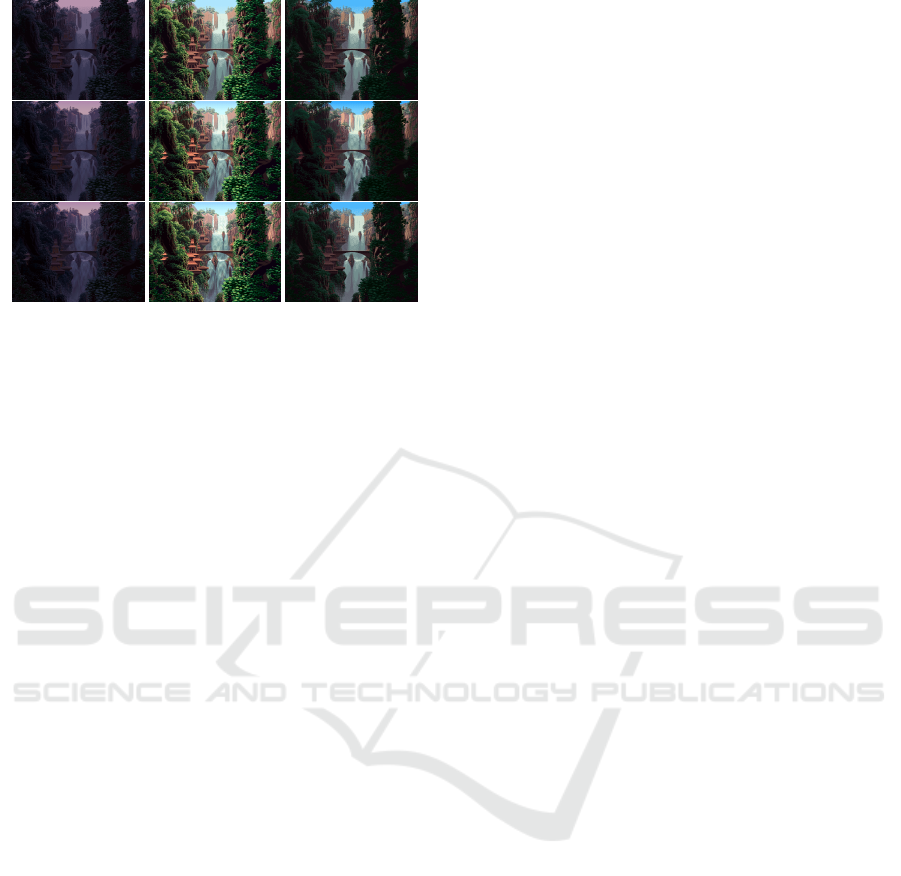
Figure 3: From top to bottom: our results with 16, 64, and

256 colors. Using the full 256 colors, our algorithm was

able to almost fully reconstruct the hand-drawn animation.

Results are good even with a reduction to 64 colors, and the

content is recognizable with as few as 16 colors.

were commonly depicted; see Figure 2. Such changes

play to the strength of palette cycling, where the col-

ors used can be radically different at different stages

of the animation.

We propose a method for automatic creation of

palette cycling animations from an input video se-

quence. We make no assumptions about the video

content, and are able to treat cases including large-

scale motion or camera movement that were ex-

tremely challenging to create by hand. Such scenarios

are not well suited to palette cycling, though. Palette

cycling is most effective for animations where there

is little camera movement and where there are color

changes over ﬁxed objects, such as time-lapse video.

In our problem, we want to optimize both the

choice of colors and the assignment of colors to pix-

els in order to best match the arbitrary input video

sequence. We achieve this by alternating two opti-

mization tasks: we dither each frame using the ﬁxed

palette for that frame, then we compute a quantiza-

tion of the image colorspace to obtain a palette to be

used in subsequent iterations. After several iterations

(around 200 for results we show) the process has con-

verged.

In this paper we propose a method that, given a se-

quence of images, creates the palettes and a shared in-

dex map that can be used to mimic handcrafted palette

cycling results. Our method alternates between creat-

ing the index map and creating palettes. We obtain

reasonable results for some typical use cases such as

sea waves and city skyline; however, for challenging

cases including large-scale motion, it is less success-

ful. Note, though, that such difﬁcult cases are intrin-

sically difﬁcult and we are not aware of handmade

examples that successfully portray this sort of con-

tent.We use an optimization process to create the ani-

mations. In an application, the palette cycling anima-

tions would be precomputed, and the resulting (very

small) index maps and palette sequences stored; at

runtime, the index map provides a lookup table into

the per-frame palettes, so the computational cost of

playback is extremely low.

2 PREVIOUS WORK

The problem of expressing an image with a small

color palette has been studied for a very long time.

Dithering was used to facilitate printing images in

newspapers, and with the advent of computer screens

was used to display gray scale images on a black and

white screen. Floyd-Steinberg (Floyd and Steinberg,

1976) algorithm dithering was one of earlier attempts

to automate the dithering process using error diffusion

to improve the results. A more recent approach (Pang

et al., 2008) to halftoning directly optimizes an en-

ergy function that estimates human perception of im-

age differences.

2.1 Dithering

Historically, halftoning algorithms were divided into

two styles: ordered dithering (Bayer, 1973), which

uses repetition of a structured pattern of thresholds

to approximate an image, and error diffusion (Floyd

and Steinberg, 1976), which processes pixels in some

order and distributed error to nearby unprocessed pix-

els. Ordered dither is fast, but often results in visible

repetition. Error diffusion is more ﬂexible and many

variants have been developed (Eschbach and Knox,

1991; Liu and Guo, 2015; Kim and Park, 2018; Xia

et al., 2021).

Error diffusion methods are capable of producing

high-quality results, but can be slow. The literature

has seen various efforts at structure preservation, with

edge preservation (Eschbach and Knox, 1991; Li,

2006; Kwak et al., 2006) and integrated optimization

systems (Pang et al., 2008; Chang et al., 2009)pro-

posed. Hardware acceleration, moving some compu-

tation to the GPU, can reduce running times (Fran-

chini et al., 2019). More recently, deep learning

methods have been applied to halftoning (Kim and

Park, 2018; Xia et al., 2021). Such methods can

be extremely effective, but are costly. Since we use

halftoning as a computation within the inner loop of

an optimization process, we require an extremely fast

halftoning technique, and have opted not to use any

of these sophisticated yet expensive methods.

GRAPP 2024 - 19th International Conference on Computer Graphics Theory and Applications

116

Work on halftoning has often been motivated by

applications in printing or e-ink, where only two col-

ors are available, or where a choice is made from a

small number of possible colors, known in advance

of the halftoning process. In our case, we can jointly

select the palette and the palette index distribution, a

comparatively little-studied problem.

Some work has been done on automated pixel

art (Gerstner et al., 2012; Inglis and Kaplan, 2012) re-

producing input images using few colors at ultra-low

spatial resolutions. While adjacent to our interests,

the main challenges here relate more to the spatial

resolution than the color reduction. That said, both

automated palette cycling and pixel art would beneﬁt

from a halftoning method tuned to the requirements

of low-resolution images with medium palette sizes

(say, 256 to 1024 colors).

2.2 Palette Creation

Palette creation, as color quantization, is a technique

for reducing the number of colors used in a digital im-

age. This process emerged with the advancement of

computers and the ability to create custom palettes for

displaying images on screen. A common approach to

creating custom palettes is through the use of cluster-

ing algorithms in color space. Examples of this type

of algorithm include median cut (Heckbert, 1982),

octree (Gervautz and Purgathofer, 1988), and self-

organizing maps (Park et al., 2016).

Later algorithms improved the quality of palette

creation. One example is the modiﬁed median

cut (Joy and Xiang, 1993), which improves on the tra-

ditional median-cut algorithm by incorporating addi-

tional information such as color similarity and human

perception of color.

Despite the effectiveness of color quantization, the

limited palette size used in our application means that

dithering is still a necessity.

2.3 Joint Dithering and Palette Creation

Dithering and palette creation are interrelated prob-

lems. Rather than solving them independently, ap-

proaching them as a joint problem can produce

improved results. Orchard and Bouman (Orchard

et al., 1991) combine binary tree palette creation

with dithering.

Ozdemir and Akarun (Ozdemir and

Akarun, 2001) combine fuzzy c-means methods with

Floyd-Steinberg dithering to create a color palette,

and then use this palette to perform quantization and

dithering as usual. Puzicha et al. (Puzicha et al., 2000)

were the ﬁrst to simultaneously perform quantization

and dithering by minimizing a cost function based on

a weighted Gaussian distortion measure, which aims

to directly simulate the human visual system. Huang

et al. (Huang et al., 2016) improve on this method by

using an edge-aware Gaussian ﬁlter to avoid soften-

ing edges in the input image. None of these meth-

ods considered the problem of palette cycling; in this

work, we jointly create a palette and dithering where

the dithered image is an index map shared across an

entire animated sequence.

3 PROPOSED ALGORITHM

Our algorithm takes an input animation sequence I

consisting of a set of frames I

; our goal is to ob-

tain an index map M and a sequence of palettes P that

together form a palette cycling approximation of the

input video. The index map has one entry per pixel,

indicating which palette entry should be used to color

that pixel; the palette sequence has one palette per

input frame, with individual per-frame palettes indi-

cated as P

. We jointly ﬁnd an index map and set

of palettes that minimize the difference between the

encoded animation and the original animation. Our

strategy is to alternate between (i) ﬁnding an index

map, given the current palette set; (ii) given the per-

pixel palette indices, determining a palette for each

frame to best match the corresponding input frame.

An overview of the process is shown in Figure 4.

Similar to Huang et al.’s method, we deﬁne a cost

function that we aim to minimize. Our cost function

is the total difference between the smoothed output

and smoothed input across all frames. We compare

smoothed frames so as to maximize the effectiveness

of the dithering; the human eye will naturally perform

some spatial integration, and we can obtain perceptu-

ally better results by smoothing compared to taking

the smallest-error result for an individual pixel. In-

deed, this is the premise underlying the entire ﬁeld of

dithering. Smoothing is done using the bilateral ﬁlter;

note that smoothing is spatial and not temporal.

Let I

be the input image of frame f , and C

the function which computes smoothing over frame

f . Further, let M/P

be the output frame when

the palette at frame P

is applied using the index

map M. Consequently, C

) and C

(M/P

) are

the smoothed versions of I

and M/P

respectively.

Given this notation, we can express the objective

function as follows:

error =

∑

||C

) −C

(M/P

)||

, (1)

where we aim to ﬁnd M and P that minimize the error.

Automated Palette Cycling Animations

117

Output Frames

Input Frames

Final Index Map

Final Palettes

Optimization loop: Alternate between

optimizing index map and palettes

Index Map

Per-Frame Palettes

Encoded sequence: global index map

plus palette for each frame

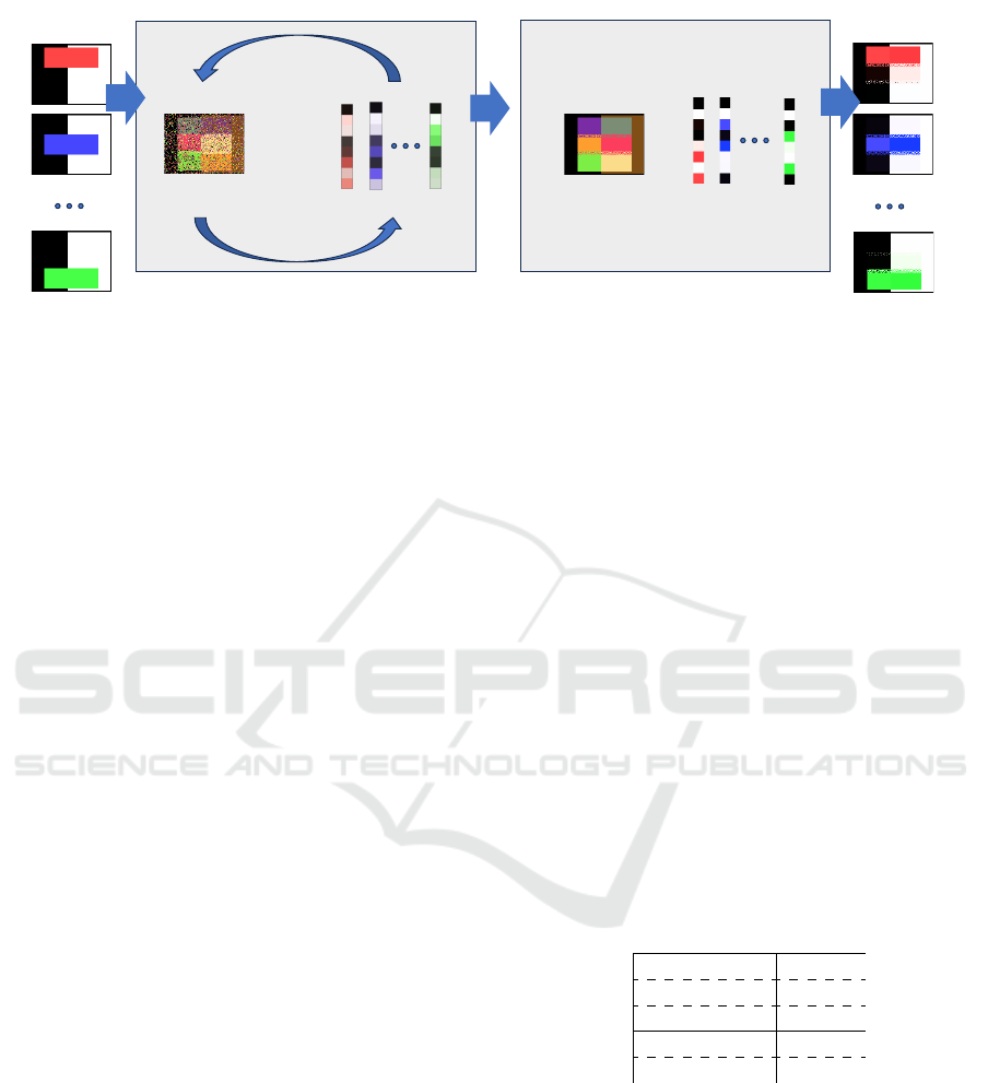
Figure 4: Overview of the process. From left to right: we begin with an input video sequence, divided into individual frames;

we create an index map and per-frame palettes and iteratively optimize them, alternating between optimizing the index map

(with ﬁxed palettes) and the palettes (with ﬁxed index map); when the optimization loop terminates, we have a ﬁnal index

map and palette set, which can be decoded into individual frames approximating the input.

3.1 Initialization

We initialize the index map with random values: with

a palette size of n, each pixel gets a value in the range

0 to n − 1. The initial palette entries are obtained by

computing, for each index in a given frame, the aver-

age color of all pixels in the original frame that share

that index. Following initialization, we repeatedly al-

ternate between updating the index map, with ﬁxed

palettes, and updating the palettes, with a ﬁxed index

map. We discuss these two steps in turn in the follow-

ing subsections.

3.2 Dithering

In this step, we assign an index to each position in

the index map, given a ﬁxed set of palettes. The ap-

proach is to modify the existing index map one entry

at a time. Inspired by simulated annealing, we make

random changes to the indices with probabilities tilted

towards the values that produce the least error. The

randomness is intended to allow the index map to es-

cape from local minima.

For each pixel, for each possible index assignment

i, we compute the associated error E

. The weight w

associated with index i is given by

= (1/E

)

(ln(γ)/ln(r))

, (2)

where γ is an iteration-dependent parameter used to

adjust the randomness during convergence, and r is

the ratio of the errors of the best and second-best

choice, used to guide the shape of the local proba-

bility distribution. The parameter γ is assigned using

a quadratic function, γ(k) = (k − µ)

+ ε, for iteration

count k and constants µ = 25 and ε = 2; the intent is to

have a large γ at the start and end of the minimization

process, weighting the best choice much more heav-

ily than the others, and a small γ for a period in the

middle, allowing a ﬂatter distribution of weights and

letting the system explore variations on an initial ap-

proximately greedy assignment.

Having computed the distribution of weights for a

given pixel, we assign an index to that pixel, choosing

randomly with probability apportioned according to

the weights. We repeat this process across all pixels

treated during this iteration.

Because our error calculation incorporates

smoothing, a change to one pixel’s index affects the

weights for nearby pixels. Our maximum smoothing

kernel is 5 × 5. We would like to use information that

is up to date when selecting indices, but also want to

take advantage of parallelism. As a compromise, we

created a schedule for changing indices, where the

index map is divided into nine interleaved regions,

repeating according to the following pattern:

1a 2a 3c 1a ...

2c 3b 1c 2c ...

3a 1b 2b 3a ...

1a 2a 3c 1a ...

. . . . ...

Regions labeled 1, 2, 3 are processed in separate

iterations, while regions a, b, c are processed sequen-

tially within a given iteration. To be precise, only in-

dices with a numerical value equal to (k mod3)+1 are

changed during iteration k. Notice how within a given

5x5 window, the central index only appears once, so

that it can be changed and evaluated independently;

other indices are considered ﬁxed. As a side effect,

since we only change one-third of the pixels within

an iteration, the index map remains relatively stable

between calculations of the per-frame palettes which

GRAPP 2024 - 19th International Conference on Computer Graphics Theory and Applications

118

helps to speed up ﬁnding the numerical solution to the

equations in palette creation.

3.3 Palette Creation

We represent the sequence of palettes

for an animation as a set of 2D matri-

ces P

∈ Rˆ(indices × channels). We con-

sider the image frames to be 3D tensors

∈ Rˆ(width × height × channels). The

palette index lookups for the animation are

represented by a single 2D integer matrix

M[x,y] ∈ Nˆ(width × height), whose entries in-

dex into the palette for each frame. We encode

the output frame as a one-hot encoded matrix

M[x,y,q] ∈ Rˆwidth × height × palette) shown in

equation 3:

M[x,y,q] =

(

1 q = M[x,y]

0 q ̸= M[x,y]

(3)

The matrix

M thus produces the sequence of out-

put frames through multiplication with the palette se-

quence. We can then express the goal of selecting a

suitable palette for frame f as the minimization of the

difference between the original frame and the output

frame:

min

||C

(

M × P

) −C

)|| (4)

As we have expressed everything in terms of lin-

ear equations, the minimization can be obtained by

solving the following overdetermined system to de-

termine P

(

M × P

) = C

). (5)

Note that equation 5 has a number of equations equal

to the number of pixels, but the number of unknowns

is only equal to the number of palette entries times the

number of color channels. Further note that we are

computing the difference of the smoothed images; to

solve for P

, we can incorporate the smoothing into a

single matrix and compute P

= (C

(

M))

−1

×C

where due to the overdetermined system, we use a

pseudoinverse and not an inverse.

Solving the system of equations can yield unreal-

izable colors; for example, they might have negative

components. One might imagine various ways of ad-

dressing this, such as rescaling the entire palette se-

quence to the legal range. We do not want to change

the entire color sequence because of a few outliers.

Instead, we identify illegal entries and modify them

individually, clamping the color components to the

permitted range, as follows:

[i] =

(

[i]

[i] in range

max(0,

[i]) ×

range

[i]|

otherwise

(6)

The collection of per-frame palettes obtained from

solving equation 5 for each frame produces a tentative

collection of colors which are used in the next round

of index selection. After several rounds of alternat-

ing global index selection and per-frame palette se-

lection, we have our output, an approximation of the

input video sequence encoded as a palette cycling an-

imation.

3.4 Additional Complications

Two ﬁnal details must be added. First, we discuss a

“palette compression” modiﬁcation, designed to free

up a few palette indices for small but visible details

in the animation. Second, we describe a schedule for

adjusting the smoothing kernel size, beginning with a

small kernel and migrating to a larger one over time;

this is done to improve performance, since a smaller

kernel can be processed more quickly, and early iter-

ations are so far from the input video that smoothing

makes little difference.

3.4.1 Palette Compression

The global error-minimizing solution may ignore

small, ephemeral details that are nonetheless percep-

tually salient. To combat this, we intermittently com-

press the palettes so as to be able to represent the

main colors with fewer palette entries. The colors thus

freed are able to be used for additional animation or

for rare but distinct colors. We opted to perform com-

pression every ﬁve iterations; the results are not very

sensitive to the frequency of compression.

Palette compression is done by computing k-

means clustering over the colors in the palette, with

a cluster count of 90% of the original palette size.

Following clustering, we update the palette and the

corresponding index maps to use the cluster centers

as the new palette entries.

Following palette compression, some indices in

the palette are now unused. We can then use them

for speciﬁc, high-impact details. We process the in-

dex map, looking for the indices that contribute the

greatest amount of error. The m unused entries in the

palette are then assigned to the m locations in the in-

dex map with largest error. At ﬁrst glance, it may

seem wasteful to use an index entry for a single pixel,

but recall that we are undertaking an iterative process

and these new indices will be available to the rest of

the index map at later iterations.

A typical outcome of the above compression and

reassignment process is for certain palette entries to

Automated Palette Cycling Animations

119

be used by small-scale repeating patterns in the video,

such as lights in windows and headlights of cars mov-

ing along a highway. Although these entries are used

very few times in the dithered image, they often rep-

resent highly salient details, such that reserving some

palette entries in this way improves the ﬁdelity of the

palette cycling animation.

3.4.2 Smoothing Schedule

We smooth using the bilateral ﬁlter with a 5 × 5

smoothing window. For each kernel, the weights

are computed per-frame and per-pixel, a moderately

costly process. We propose starting with a kernel

diameter of 1 at the beginning, effectively disabling

smoothing, and gradually increasing the kernel size

as the algorithm approaches the maximum iteration

count. In this way, we are able to process the early

iterations more quickly, while performing the ﬁnal

rounds of iteration using the full kernel; typically we

ran 220 iterations and had the full kernel size from it-

eration 170 onward. This smoothing schedule saved

computation; see Table 1 for per-iteration times for

a sample animation. Empirically, beginning with a

smaller kernel had no negative effect on the ﬁnal er-

ror; some quantitative results are provided in the fol-

lowing section.

Table 1: Average time per iteration given different kernel

sizes. Data is given for the tower animation with 256 palette

entries.

kernel diameter (pixels) 1 5 9 21

time per iteration (seconds) 2.73 8.12 10.63 10.40

4 RESULTS

We tested our method on some types of scenes that

have been traditionally animated using handcrafted

palette cycling. In addition, we tested on scenar-

ios such as human-ﬁgure movement and large-scale

motion, where we have not seen palette cycling an-

imations made by hand. In this section, we ﬁrst re-

port quantitative measures, followed by examples and

qualitative evaluation of different scenarios in the in-

put video. Out examples include repetitive motion,

time-lapse video, and more difﬁcult cases involving

large-scale motion and moving backgrounds or view-

points.

4.1 Error Proﬁles

To evaluate the results, we computed an error mea-

sure, comparing each frame in the algorithm result

against its counterpart in the original image. As men-

tioned previously, we use smoothed versions of both

images, useful in assessing dithered images. The

smoothing uses the bilateral ﬁlter with ς

= 100 and

= 500.

We use the towers example as a standard bench-

mark for many evaluations. This animation consists

of 150 frames at 320x570 resolution. Its palette se-

quence is shown in Fig 5, while Figure 6 compares

two frames of the source video against the recon-

structed images.

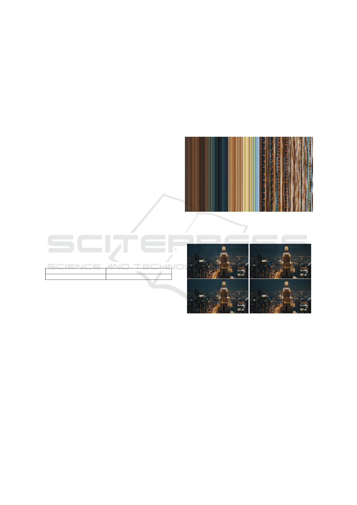
Figure 5: Visualization of palette sequence for the tower

example. Palettes are horizontal stripes; time progresses

top to bottom. Notice the blinking lights, visible as dashed

lines in some indices.

Figure 6: Two sample frames from the tower example.

Above: original frames; below: palette cycling versions.

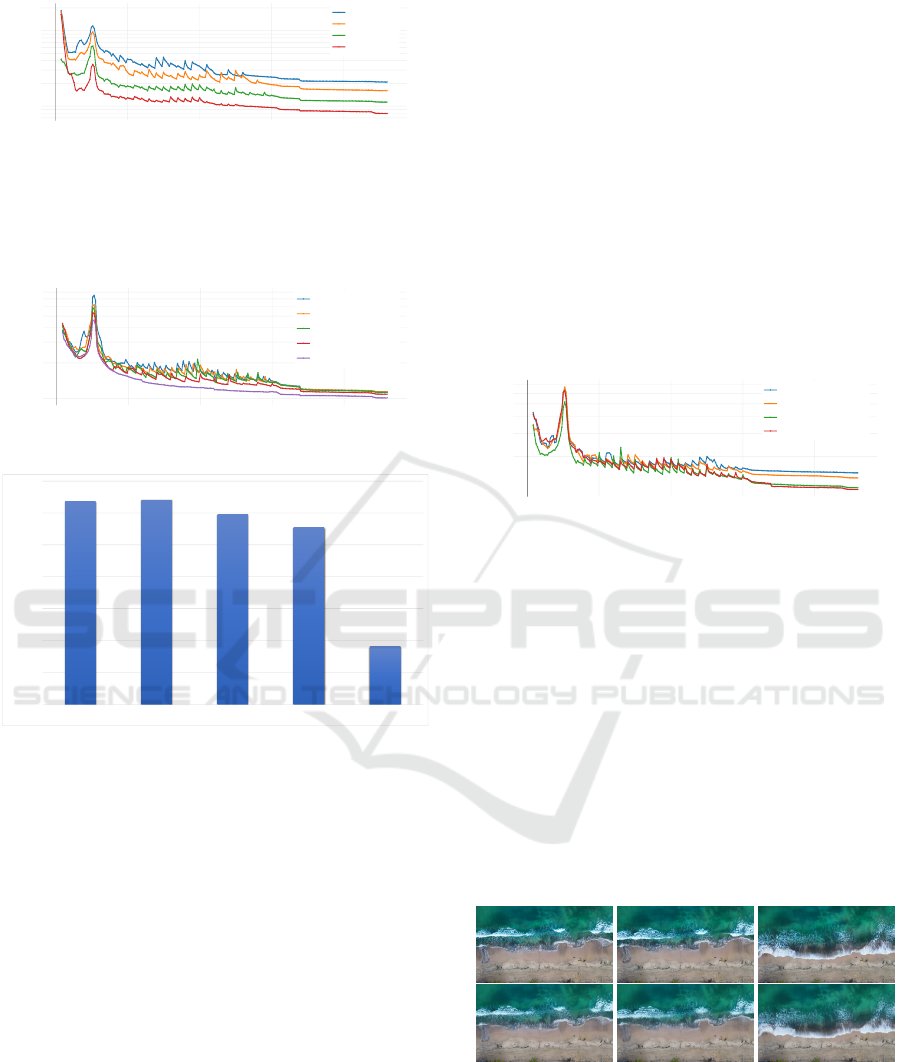
Figure 7 shows the error measure as the index map

and palettes are reﬁned over many iterations. Unsur-

prisingly, larger palettes produce smaller absolute er-

ror. The spikes in the error are aligned with instances

of palette compression, when a few palette entries are

repurposed to cover small details, often animated de-

tail. The spikes quickly subside as the new indices are

used for additional pixels, as previously described.

In Figure 8, we can see that when the compres-

sion runs less frequently, the average error across all

frames decreases. However, the number of colors

used for animation will decrease as well; see Figure 9.

A larger number of animated colors yields greater vi-

sual interest and higher ﬁdelity for time-varying pix-

GRAPP 2024 - 19th International Conference on Computer Graphics Theory and Applications

120

0 50 100 150 200

100k

tower(32)

tower(64)

tower(256)

tower(1024)

Figure 7: The convergence rate as compared between dif-

ferent palette sizes.

els, which are highly salient perceptually. Balancing

between these two considerations, we decided to ap-

ply compression every 5 frames.

0 50 100 150 200

100k

200k

300k

400k

500k

600k

700k

800k

Every 4th

Every 5th

Every 7th

Every 10th

No Compression

Figure 8: The effect of compression on the error.

100

120

140

Every 4th Every 5th Every 7th Every 10th No Compression

Number of Animated Entries in Palette

Figure 9: The effect of compression on the number of an-

imated colors in the palette. A larger number of animated

colors indicates more resources expended on animated por-

tions of the video, which is desirable.

As shown in Figure 10, using our progressive ker-

nel size plan has an almost negligible impact on the ﬁ-

nal error values, and even potentially a beneﬁt. Using

the smaller kernel sizes in the initial iterations may

prevent the algorithm from getting stuck in a local op-

timum, producing even lower error values when the

progressive method switches to 5x5 kernel sizes at it-

eration 170.

Table 2 shows summary statistics for selected in-

put videos and conﬁgurations. Error is reported as

a per-pixel average, i.e., normalized for video length

and frame size; timing ﬁgures are per iteration. The

computation time is linear in number of frames and in

number of pixels.

The table shows signiﬁcant increases in cost for

large palette sizes (1k and higher) with only modest

gains in video quality. Simpler animations such as

the moon can obtain excellent results even with small

palettes, while challenging results such as the ranger

have high error. When frames in the animation are

signiﬁcantly different, it is more difﬁcult to encode

them into a single index map; thus, the “random”

example (where the frames blend between unrelated

images) has the highest error, even though perceptu-

ally this result was unobjectionable, probably because

viewers have no expectation of consistent motion in

this scenario. The reader will ﬁnd other observations

of interest in consulting the data given in the table.

In the following subsections, we discuss some

speciﬁc videos and give a qualitative assessment of

the results. We attempted to show a range of difﬁculty

levels, ranging from conventional use cases of natu-

ral motion and time-lapse video through challenging

cases involving human faces and large-scale motion.

0 50 100 150 200

100k

200k

300k

400k

500k

600k

700k

1x1 Kernel

3x3 Kernal

5x5 Kernel

Progressive Kernel

Figure 10: The effect of different kernel sizes on error.

4.2 Natural Motion

Repetitive cyclical motions such as water waves, a

waving ﬂag, or falling snow are good candidates for

palette cycling animations. Handcrafted palette cy-

cling often featured repetitive motions, especially in-

volving water. We show two examples of animated

water in Figures 11 and 12. The recreated seashore

adequately reproduces the motion; ﬁne details are

lost, though an impression of water remains. The

moon example has a particularly good outcome be-

cause of the limited color range of the input, mean-

ing that many palette entries could be used for color

change as opposed to distinct colors.

Figure 11: Shore example. Above: original frames; below:

recreated frames. The patterns of sea waves are reasonably

regular, which helps the algorithm capture the wave move-

ments.

Automated Palette Cycling Animations

121

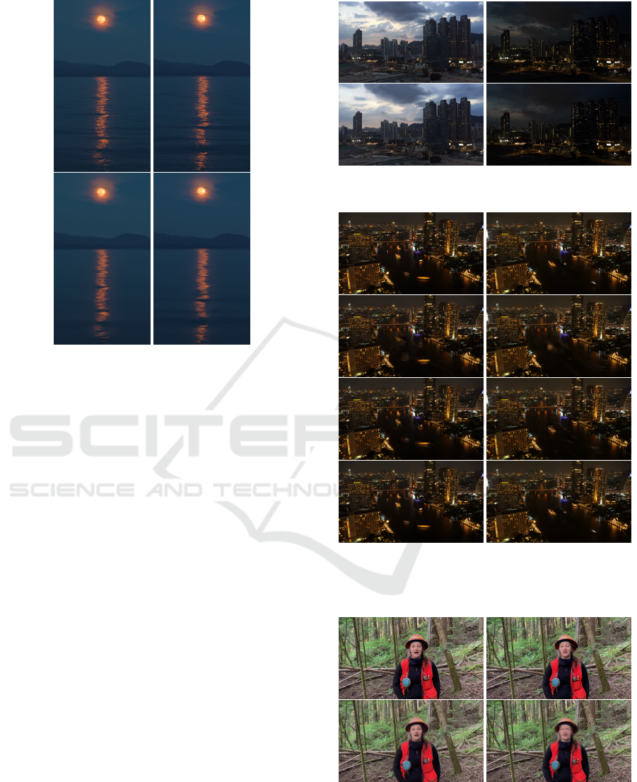
Figure 12: Moon example. Above: original frames; below:

recreated frames. The original has quite limited color vari-

ation, allowing many palette entries to be used for motion.

4.3 Time Lapse

Time-lapse video is particularly well suited to palette

cycling. Because each frame has its own palette,

large-scale coordinated color changes are easy to

manage. The hotels example shown in Figure 13

provides an example: even though the entire scene

changes color, the underlying structures do not

change and many pixels have the same color trajec-

tory. Consequently, the algorithm manages to capture

all the changes even though virtually no pixel is static.

Notice how the palette gradually darkens as the ani-

mation progresses.

Figure 14 shows an example combining motion

and large-scale change. The large-scale lighting

changes are handled well; local motion is more de-

manding, though, and the water trafﬁc is reproduced

in an impressionistic rather than entirely strict fash-

ion. In the full animation (see supplemental material),

small details such as blinking lights can be seen to be

preserved.

4.4 Larger-Scale Motion

Large-scale motion is a particular challenge for

palette cycling. Whenever two pixels differ at any

point in the animation, they need different indices

in the index map so that they can be distinguished.

Smooth motion therefore requires a very large palette;

Figure 13: Hotels example. The large-scale lighting

changes are represented elegantly through palette cycling.

Figure 14: City-river example. 1st row: original frames;

2nd row: encoded frames with 256 colors. 3rd row: en-

coded frames with 1024 colors, 4th row: encoded frames

with 4096 colors.

Figure 15: Ranger example (Total of 100 frames): The orig-

inal video had a shaky background, forcing the algorithm to

expend a large fraction of palette entries depicting the mo-

tion. This is especially evident when looking at the sides of

the tree trunks: notice the uniform colored bands parallel to

the trees. Additionally, the fast, unpredictable movement of

head and facial features was not captured well.

GRAPP 2024 - 19th International Conference on Computer Graphics Theory and Applications

122

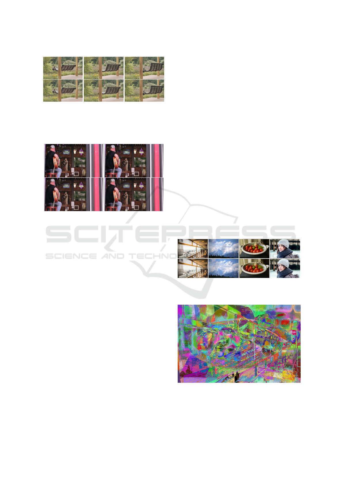
Figure 16: Swing example (Total of 40 frames): The swing

is a large object with signiﬁcant movement, a challenging

case. In the rightmost and leftmost frames, the swing is

relatively stationary and is clearly depicted. In the middle

frame, however, the speed is higher and it becomes quite

blurry.

Figure 17: Guitar example. Above: original frames; below:

reconstructed frames with 256 colors. The color variety and

camera movement make this a particularly challenging case.

with smaller palettes, the motion itself becomes visi-

bly quantized, with a choppy appearance resembling

a low frame rate. The resulting spatial quantization of

movement is a reﬂection of the underlying index map.

The swing animation demonstrates the outcome

when our process is applied to videos containing

large-scale coherent motion. The swing appears to

jump between positions. Much of the palette is con-

sumed by the varied colors in the background, leaving

only a fraction to encode the motion. Nonetheless, the

motion is recognizable, and because of the clear back-

ground, the context is easily identiﬁable.

The ranger animation exhibits similar choppiness

and ghosting. This is a more difﬁcult case than the

swing because the camera is moving as well; further,

because the subject of the animation is human, we as

human observers are less tolerant of errors.

4.5 Moving Backgrounds

The ranger animation combines large-scale motion

with a moving camera, or equivalently, a moving

background. Non-static backgrounds are a signiﬁcant

challenge for palette cycling animations, since the in-

dex map has to manage all color trajectories in the

image. Where many pixels share the same trajectory,

the problem is simpliﬁed; in cases like this one, where

many pixels have unique trajectories, the problem is

magniﬁed, and multiple trajectories must be merged.

The guitar sequence further demonstrates the chal-

lenges posed by a moving camera. The result is

grainy as the small palette struggles to cope with the

high number of trajectories, falling back on dithering.

The guitar sequence contains substantial color vari-

ation within a single frame, further raising the chal-

lenge. Nonetheless, despite noticeable deﬁciencies in

the palette cycling animation, the main objects and ac-

tions are recognizable from the result. This sequence

is considerably more difﬁcult than anything attempted

with previous manual approaches.

4.6 Image Transitions

As a curiosity, we also demonstrate a result from

blending between a sequence of static images. The

images themselves are shown in Figure 18 and the in-

dex map resulting from the optimization can be seen

in Figure 19. The palette cycling animation is pro-

vided in the supplemental material. Despite the dis-

similarity between the images, a single index map

is able to capture both the images themselves and a

smooth transition between them, with the frames re-

producing the images (Figure 18, lower row) being

very close to the originals.

Figure 18: Sequence of static images forming the basis of

an animation. Above: original images. Below: images re-

produced from common index map, palette size 256.

Figure 19: Visualization of index map for the random ex-

ample.

Automated Palette Cycling Animations

123

Table 2: Processing time and ﬁnal error for various conﬁgurations.

Conﬁguration Time Error

Video Dimensions Frames Palette Size Palettes Dithering Total (normalized)

Tower 529x320 150

32 4.81 0.69 5.49 1.47

64 5.51 1.08 6.58 1.13

256 9.26 3.19 12.44 0.80

River 853x480 202

32 17.01 1.92 18.93 2.55

256 32.49 8.95 41.44 1.58

1024 102.51 35.90 138.41 1.11

4096 433.11 154.05 587.16 0.74

M.Ferrari 640x480 418

16 23.42 2.08 25.49 3.97

64 28.57 4.50 33.07 0.79

256 38.91 15.26 54.17 0.03

Moon Reﬂection 720x405 302 32 11.78 1.94 13.72 1.54

Random 1024x650 4

32 1.55 0.30 1.85 13.05

64 1.70 0.36 2.06 10.01

Ranger 1138x640 99 256 35.42 8.06 43.48 3.92

Shore 1280x720 40 64 9.09 1.48 10.57 4.16

5 DISCUSSION

Here we recount some design advice summarizing

the lessons learned from our experiences with au-

tomated palette cycling animations. In general, our

method succeeds at encoding an input video into the

restricted form of a palette cycling animation. How-

ever, not all scenes are equally well suited to such en-

codings. Scenes with relatively static structures, such

as landscapes or cityscapes, can be encoded well even

when the lighting changes dramatically; the per-frame

palettes handle arbitrary lighting changes as long as

the pixel trajectories of multiple locations are coor-

dinated. Animations with large empty regions of the

image (e.g., a uniform sky or a ﬂat, untextured back-

drop) result in superior-quality encodings since more

palette entries can be reserved for encoding motion.

Conversely, large-scale motion such as the ap-

parent motion resulting from moving backgrounds is

more difﬁcult. The output videos begin to exhibit vis-

ible degradation compared to the source, since man-

aging the uncoordinated color changes requires many

separate indices. Considerably larger palette sizes

would be required in order to get substantial improve-

ments. and can result in severe blurring. Animations

that mix large-scale motion and color variation are

particularly challenging, since both phenomena will

place demands on our limited supply of palette en-

tries; again, blurring is a likely outcome. A relatively

simple yet problematic animation is a pan over a com-

plex background (the “Ken Burns effect”), to which

palette cycling as presently conceived is particularly

poorly suited. More generally, animated ﬁne details

are likely to suffer loss in encoding, with facial fea-

tures being challenging due to a combination of mo-

tion, color variation, and sensitivity of observers.

We used a single index map for the entire se-

quence. For short sequences, even radically differ-

ent frames can be well encoded (e.g., see the “ran-

dom” sequence). As the input becomes longer, the

output quality will degrade; the rate of quality loss

depends on the variability of frames, with more con-

sistency between frames being easier to handle. For

very long sequences, we recommend storing multiple

index maps rather than relying on a single map.

Palette cycling is of greatest value when memory

constraints are severe. It is natural to wonder what

proportion of the memory usage is due to the index

map and what proportion is consumed by the palettes.

The memory footprint of an encoded video depends

on the frame dimensions and the palette size, and is

not affected by the video content. Consider a video

with 100 frames, each 0.25 megapixels, and a palette

size of 256; the encoded video would require 0.25 MB

for the index map and 100×256 ×3 bytes for the per-

frame palettes, for a total size of 0.33 MB. For com-

parison, an animated GIF with the same parameters

(100 frames at 0.25 megapixels each) would require

100 × 0.25 = 25 MB, plus a negligible additional ex-

pense for the global palette. The animated GIF can

be compressed to reduce ﬁle size, but must be decom-

pressed for playback.

6 CONCLUSION

Palette cycling is an animation technique which uses

a ﬁxed set of indices throughout the entire sequence

of frames, with a per-frame palette. By changing

GRAPP 2024 - 19th International Conference on Computer Graphics Theory and Applications

124

the palette from frame to frame, lighting changes and

apparent motion can be induced. In this paper, we

demonstrated an optimization-based method for cre-

ating palette-cycling animations from arbitrary input

videos. Our technique involves alternating between

ﬁnding a set of per-frame palettes given a set of palette

indices, and then ﬁnding the pixel indices given a

ﬁxed set of palettes. While many handcrafted palette

animations have been created historically, this paper

is the ﬁrst to automate palette cycling.

The method produces quite good results for tradi-

tional use cases such as scenes with minor natural mo-

tion or time-lapse videos. Intrinsically difﬁcult sce-

narios including large-scale motion and moving back-

grounds are less successful and offer opportunities for

further investigation.

The present method takes only an input video,

without annotations. Better results might be achieved

by allowing a user to mark regions of interest, and pri-

oritizing ﬁdelity in those areas while discounting error

outside the important regions. Of course, the region

of interest determination could also be automated. It

might also be worthwhile to preprocess the video to

reduce the number of colors, rather than strictly rely-

ing on dithering; for example, L0 quantization could

be employed to reduce gradients.

We concentrated on photorealistic videos, while

historical palette cycling used pixel art. A possible

direction would be to jointly construct a pixel art styl-

ization and a palette cycling animation from an input

video. Further, the animation could itself be stylized,

as in handcrafted palette animations: one might imag-

ine artist-drawn tracks for particle effects or lighting

which could build on an input scene or video. Over-

all, we hope that this paper can spark renewed interest

in the fascinating medium of palette cycling.

ACKNOWLEDGEMENTS

Thanks to the GIGL group for helpful suggestions as

this project developed. The project received ﬁnancial

support from Carleton University and from NSERC.

We want to thank Mark Ferrari for his kind words of

encouragement as we were beginning this project and

for his permission to reproduce frames from the jun-

gle animation, shown in Figure 2.

REFERENCES

Bayer, B. E. (1973). An optimum method for two-level ren-

dition for continuous tone pictures. Proc. of IEEE Int’l

Communication Conf., 1973, pages 2611–2615.

Chang, J., Alain, B., and Ostromoukhov, V. (2009).

Structure-aware error diffusion. ACM Trans. Graph.,

28(5):1–8.

Eschbach, R. and Knox, K. T. (1991). Error-diffusion al-

gorithm with edge enhancement. J. Opt. Soc. Am. A,

8(12):1844–1850.

Floyd, R. W. and Steinberg, L. (1976). An adaptive algo-

rithm for spatial greyscale. Proceedings of the Society

for Information Display, 17(2):75–77.

Franchini, G., Cavicchioli, R., and Hu, J. C. (2019).

Stochastic ﬂoyd-steinberg dithering on GPU: image

quality and processing time improved. In 2019 Fifth

International Conference on Image Information Pro-

cessing (ICIIP), pages 1–6.

Gerstner, T., DeCarlo, D., Alexa, M., Finkelstein, A., Gin-

gold, Y., and Nealen, A. (2012). Pixelated image ab-

straction. In Proceedings of the tenth annual sympo-

sium on non-photorealistic animation and rendering

(NPAR 2012), pages 29–36.

Gervautz, M. and Purgathofer, W. (1988). A simple

method for color quantization: Octree quantization. In

Magnenat-Thalmann, N. and Thalmann, D., editors,

New Trends in Computer Graphics, pages 219–231,

Berlin, Heidelberg. Springer Berlin Heidelberg.

Heckbert, P. (1982). Color image quantization for frame

buffer display. In Proceedings of the 9th Annual Con-

ference on Computer Graphics and Interactive Tech-

niques, SIGGRAPH ’82, page 297–307, New York,

NY, USA. Association for Computing Machinery.

Huang, H.-Z., Xu, K., Martin, R. R., Huang, F.-Y., and Hu,

S.-M. (2016). Efﬁcient, edge-aware, combined color

quantization and dithering. IEEE Transactions on Im-

age Processing, 25(3):1152–1162.

Inglis, T. and Kaplan, C. (2012). Pixelating vector line art.

In Proceedings of the tenth annual symposium on non-

photorealistic animation and rendering (NPAR 2012),

pages 21–28.

Joy, G. and Xiang, Z. (1993). Center-cut for color-image

quantization. The Visual Computer, 10(1):62–66.

Kim, T.-H. and Park, S. I. (2018). Deep context-aware de-

screening and rescreening of halftone images. ACM

Trans. Graph., 37(4).

Kwak, N.-j., Ryu, S.-p., and Ahn, J.-h. (2006). Edge-

enhanced error diffusion halftoning using human vi-

sual properties. In 2006 International Conference

on Hybrid Information Technology, volume 1, pages

499–504.

Li, X. (2006). Edge-directed error diffusion halftoning.

IEEE Signal Processing Letters, 13(11):688–690.

Liu, Y.-F. and Guo, J.-M. (2015). Dot-diffused halftoning

with improved homogeneity. IEEE Transactions on

Image Processing, 24(11):4581–4591.

Orchard, M. T., Bouman, C. A., et al. (1991). Color quan-

tization of images. IEEE transactions on signal pro-

cessing, 39(12):2677–2690.

Ozdemir, D. and Akarun, L. (2001). Fuzzy algorithms for

combined quantization and dithering. IEEE Transac-

tions on Image Processing, 10(6):923–931.

Automated Palette Cycling Animations

125

Pang, W.-M., Qu, Y., Wong, T.-T., Cohen-Or, D., and Heng,

P.-A. (2008). Structure-aware halftoning. ACM Trans.

Graph., 27(3):1–8.

Park, H. J., Kim, K. B., and Cha, E.-Y. (2016). An ef-

fective color quantization method using octree-based

self-organizing maps. Intell. Neuroscience, 2016.

Puzicha, J., Held, M., Ketterer, J., Buhmann, J. M., and

Fellner, D. W. (2000). On spatial quantization of

color images. IEEE Transactions on image process-

ing, 9(4):666–682.

Xia, M., Hu, W., Liu, X., and Wong, T.-T. (2021). Deep

halftoning with reversible binary pattern. In 2021

IEEE/CVF International Conference on Computer Vi-

sion (ICCV), pages 13980–13989.

GRAPP 2024 - 19th International Conference on Computer Graphics Theory and Applications

126