
Numerical Evaluation of the Image Space Reconstruction Algorithm
Tomohiro Aoyagi
a
and Kouichi Ohtsubo
Faculty of Information Science and Arts, Toyo University, 2100 Kujirai, Saitama, Japan
Keywords: X-ray CT, PET, Image Reconstruction, ISRA, Steepest Descent.
Abstract: In medical imaging modality, such as X-ray computerized tomography (CT), positron emission tomography
(PET) and single photon emission computed tomography (SPECT), image reconstruction from projection is
to produce an image of a two-dimensional object from estimates of its line integrals along a finite number of
lines of known locations. The method of tomographic image reconstruction from projection can be formulated
with the Fredholm integral equation of the first kind, mathematically. It is necessary to solve the equation.
But it is difficult in general to seek the strict solution. By discretizing the image reconstruction problem, we
applied the image space reconstruction algorithm (ISRA) to the problem and evaluated the image quality. We
computed the normalized mean square error (NMSE) in reconstructed image. We have shown that the error
decreases with increasing the number of detectors, views and iterations. In addition, the effect of the relaxation
parameter, the weighting factor and the noise to the reconstructed image are analysed.
1 INTRODUCTION
In medical imaging modality, such as X-ray
computerized tomography (CT), positron emission
tomography (PET) and single photon emission
computed tomography (SPECT), image
reconstruction from projection is to produce an image
of a two-dimensional object from estimates of its line
integrals along a finite number of lines of known
locations (Herman, 2009; Kak et al., 1998; Imiya,
1985). PET or SPECT is intrinsically a three-
dimensional imaging technique and determines the
distribution of a radiopharmaceutical in the interior of
an object by measuring the radiation outside the
object in a tomographic fashion (Bendriem et al.,
1998). The method of tomographic image
reconstruction from projection can be formulated by
the Fredholm integral equation of the first kind,
mathematically. Since observed data can be
discretized experimentally, it is necessary to
discretize the equation to solve it with digital
processing. Because of the ill-posed nature, it is
difficult to solve strictly this integral equation. Up to
now many image reconstruction methods have been
proposed by the research development regardless of
imaging modality (Stark, 1987; Natterer et al., 2001).
In general inverse problems, the regularization of
a
https://orcid.org/0000-0002-7268-9826
linear ill-posed problems has been derived and
revealed the properties (Daniel 2021; Ronny et al.,
2019; Simon et al., 2022).
It is possible to divide image reconstruction
methods into two methods, transform and iterative.
Transform methods are based on discrete
implementations of analytic solution and give a one-
step solution which is directly calculated from the
observed data. Iterative method can incorporate the
discrete nature of the data sampling and
reconstruction problem and typically some statistical
model of the data acquisition process.
The image space reconstruction algorithm (ISRA)
which is one of the iterative algebraic reconstruction
methods, has been shown to be a non-negative least
squares estimator and was introduced as an
alternative image reconstruction method for PET
(Depierro, 1987; Iniyatharasi et al., 2015). By
modifying the weighted least squares objective
function, a more general form of the ISRA has been
derived and the relation between ISRA and the
maximum likelihood expectation maximization (ML-
EM) has been revealed and shown the convergence
property (Depierro, 1993; Reader, 2011).
However, the effect of discretizing an image
reconstruction model and its parameter have been not
revealed sufficiently. In this paper, by discretizing the
78
Aoyagi, T. and Ohtsubo, K.
Numerical Evaluation of the Image Space Reconstruction Algorithm.
DOI: 10.5220/0012432100003651
Paper published under CC license (CC BY-NC-ND 4.0)
In Proceedings of the 12th International Conference on Photonics, Optics and Laser Technology (PHOTOPTICS 2024), pages 78-85
ISBN: 978-989-758-686-6; ISSN: 2184-4364
Proceedings Copyright © 2024 by SCITEPRESS – Science and Technology Publications, Lda.

image reconstruction problem, we applied ISRA to
the problem and evaluated the image quality. We
computed the normalized mean square error (NMSE)
in reconstructed image. We have shown that the error
decreases with increasing the number of detectors,
views and iterations. By introducing the new
weighting factors which is the linear combination of
the expected data vector from a given image estimate,
measured data vector and constant term, new update
method was derived. Also, we have shown the effect
of the relaxation parameter and noise to the
reconstructed image.
2 REVIEW OF ISRA
The observed data g=
g
can be viewed as the
components of a vector which will be called the data
vector or an element in the finite dimensional Hilbert
space. The unknown characteristics of the sample,
denoted by f=
f
, can be called the object of its
physical nature. Image reconstruction problems or
imaging system models can be formulated by using
the matrix notation (Bertero et al., 1985; Bertero et
al., 1988).
g=Af
(1)
The linear operator A is an 𝑁×𝑀 real matrix 𝐴=
a
.
Let us consider the following weighted least-
squares objective function, such that,
Φ
f
=
1
2
g
−𝑝
𝑤
,
(2)
where the estimated data from a given image estimate
f
are given by
𝑝
=𝑎
f
+𝛼
.
(3)
𝛼
can be of signal-independent noise. Now, we seek
a better estimate of f, which reduces the evaluation of
the objective function or satisfies the minimum of the
objective function. This can be achieved by taking
partial derivatives with respect to f.
𝜕
𝜕
f
Φ
f
=−
𝑎
g
−𝑝
𝑤
.
(4)
The right-hand side of eq. (4) can be of an image
which is the backprojection of weighted expected
data minus the backprojection of the weighted
projection data.
𝜕
𝜕f
Φ
f
=𝑎
𝑝
𝑤
−𝑎
g
𝑤
(5)
The general iteration scheme to minimize the
objective function (2) can be derived by subtracting a
variably-scaled amount of this gradient image.
f
=f
−𝛽
𝑎
𝑝
𝑤
−𝑎
g
𝑤
(6)
This is the same method of steepest descent which is
the most widely used descent procedure for
minimizing an objective function (Luenberger, 1969;
Luenberger, 2003). If the following scaling is chosen
for a given iteration 𝑘,
𝛽
=
f
∑
𝑎
𝑝
𝑤
,
(7)
the iterative update can be obtained.
f
=f
∑
𝑎
g
𝑤
∑
𝑎
𝑝
𝑤
.
(8)
Moreover, if the wights are chosen to be 𝑤
=1, then
ISRA can be obtained, such that,
f
=f
×
∑
𝑎
g
∑
𝑎
〈
𝒂
,f
〉
,
(9)
where
〈
∙,∙
〉
indicates the inner products in Hilbert
space.
3 NUMERICAL COMPUTATIONS
3.1 Discretization of Image
Reconstruction Problem
To confirm the effectiveness of the method, computer
simulations have been carried out. A Cartesian grid of
the square observation plane, called pixels, is
introduced into the region of interest (ROI) so that it
covers the whole observation plane that has to be
reconstructed. The pixel as numbered as follows: the
top left corner pixel is set to 1and bottom right corner
is numbered as M with Raster scanning. The object to
be reconstructed is approximated to the one that takes
a constant uniform value f
throughout the 𝑗-th pixel,
for 𝑗=1,2,⋯,M. Consequently, the vector 𝐟=
Numerical Evaluation of the Image Space Reconstruction Algorithm
79
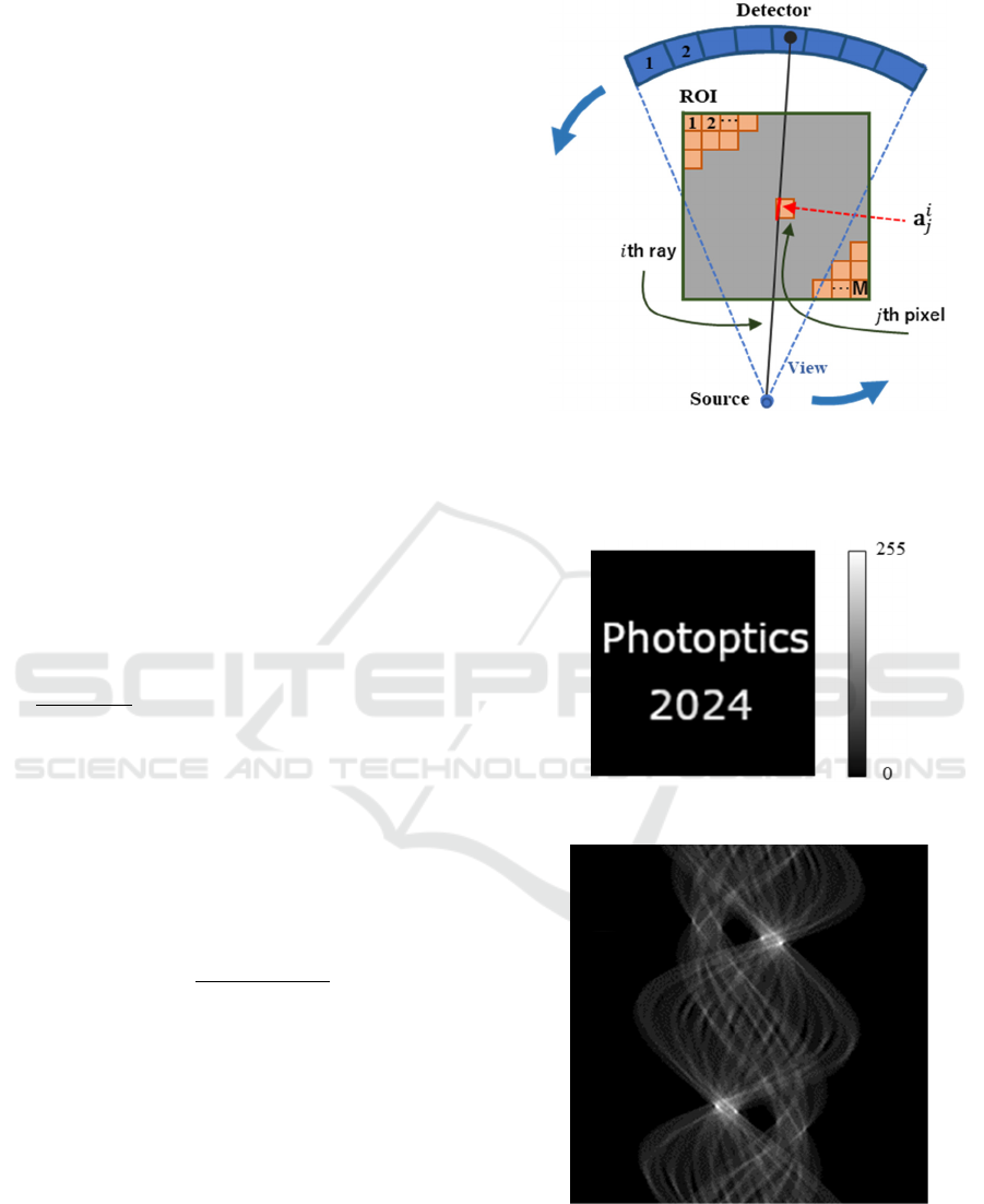
f
in ℝ
(the m-dimensional Euclidean space) is
the discretized version of the object (Censor et al.,
2008). For our simulations we assumed the fan beam
scanner in data collection mode. It consists of a single
source and multiple detectors combination which
rotates around ROI. The detector-array can be
discretized equidistantly. The set of all lines for which
line integrals are estimated can be divided into D lines
in each combination. We assumed projection angle
θ=
0,2𝜋
, and it is discretized at even. The total
number of the angles is V. It means the number of
views per 360
∘
. The total number of all discretized
line is N, which define the line of response (LOR),
such that,
𝑁=𝐷×𝑉. (10)
We set the left detector element to 1 at θ=0 and the
right detector element to N at last View. Thus 𝑖
indicates any detector elements and 𝑖=1,2,⋯,𝑁.
Consequently, the vector 𝐠=
g
in ℝ
is the
discretized version of the line integrals. We denote
the length of intersection of the 𝑖-th line with the 𝑗-th
pixel by a
, for all 𝑖=1,2,⋯,𝑁 , 𝑗=1,2,⋯,𝑀 .
Figure 1 shows the discretized model of the image
reconstruction problem.
The ISRA is the following iterative scheme.
Algorithm.
Step 1 (Initialization):
f
∈ℝ
∖
𝟎
.
Step 2: Compute the backprojection of projection
data.
h
=𝑎
g
.
(11)
Step 3 (Iterative step): Given f
and fixed the
relaxation parameter 𝛾
, compute
f
=f
×
h
∑
𝑎
〈
𝒂
,f
〉
.
(12)
3.2 Text Based Phantom
Our first image is a text based phantom. Figure 2
shows its original test image 1, discretized 128×128
pixels and 8 bit/pixel. Figure 3 shows the projection
data of the original test image 1. The number of
detectors per view is 200. The number of views per
360° is 200. Figure 4 shows the reconstructed images
by ISRA. In this case, iteration number is 30. The
number of detectors per view is 200. The number of
views per 360
∘
is 200. Initial data is a uniform image
of 0.1, 0.1=f
∈ℝ
. The relaxation parameter is
the unit.
Figure 1: The fully-discretized model of the image
reconstruction problem in 2-dimensional space. Fan beam
scanning mode (single source, multiple detector, translate-
rotate).
Figure 2: The original test image 1(128×128 pixels, 8bpp).
Figure 3: The projection data, Sinogram of the original
image in Fig. 2. 200 detectors / view, 200 views / 2π and
8bpp. Noise free.
PHOTOPTICS 2024 - 12th International Conference on Photonics, Optics and Laser Technology
80
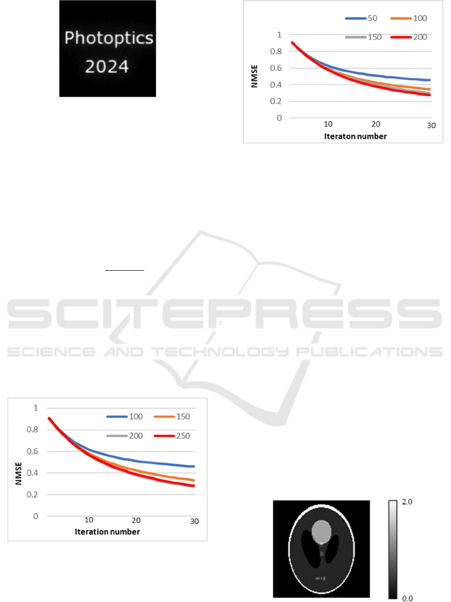
Figure 4: The reconstructed image by ISRA after 30
iterations. Initial image is a uniform image of 0.1. The
relaxation parameter 𝛾
=1.0.
To confirm the effect of number of detectors per
view, we computed the reconstructed image with its
variations from 100 to 250. Figure 5 illustrates the
plots of the normalized mean square error versus
iteration number. In this case, we set the number of
views per 360
∘
equal to 200 and the relaxation
parameter the unit. Initial data is a uniform image of
0.1, 0.1=f
∈ℝ
. Iteration number is up to 30. The
normalized mean square error (NMSE) is defined by
NMSE
𝑘
=
‖
f
− f
‖
‖
f
‖
,
(13)
where 𝐟
is the image after 𝑘’th iteration step and 𝐟 is
the original image.
‖
∙
‖
indicates the ℓ
-norm. From
Fig. 5 we can see that the error decreases with
increasing the number of iterations and the error
decreases as a whole with increasing the number of
detectors.
To confirm the effect of number of views per
360
∘
, we computed the reconstructed image with its
variations from 50 to 200.
Figure 5: Plots of normalized mean square error versus
iteration number. 200 views. Initial image is a uniform
image of 1.0. Relaxation parameter is the unit. The number
of detectors / view are changed from 100 to 250.
Figure 6: Plots of normalized mean square error versus
iteration number. 200 detectors / view. Initial image is a
uniform image of 1.0. Relaxation parameter is the unit. The
number of views are changed from 50 to 200.
In this case, we set the number of detectors per view
200 and the relaxation parameter the unit. Initial data
is a uniform image of 0.1, 0.1=f
∈ℝ
. From Fig.
6 we can see that the error decreases with increasing
the number of iterations. From Fig. 5 and Fig. 6, it is
more important that if the number of detectors, views
and iterations can be increased, NMSE can be
decreased.
3.3 Head Phantom
Our original test image 2 is 2-dimensional numerical
phantom which is the well-known Shepp and Logan’s
head phantom and models cross section of the human
head (Kak et al., 1998). This phantom is a
superposition of 10 ellipses. Figure 7 shows its test
image 2, discretized 128×128 pixels, 8 bit/pixel.
Figure 8 shows the projection data of the original test
image 2. The number of detectors per view is 200.
The number of views per 360° is 200. Figure 9 shows
the reconstructed images by ISRA. In this case,
iteration number is 50. The number of detectors per
view is 200. The number of views per 360
°
is 200.
Initial data is a uniform image of 1.0, 1.0=f
∈ℝ
.
The relaxation parameter is the unit.
Figure 7: The original test image 2(128×128 pixels, 8bpp).
Numerical Evaluation of the Image Space Reconstruction Algorithm
81
Figure 8: The projection data, Sinogram of the original
image in Fig. 7. 200 detectors / view, 200 views / 2π and
8bpp. Noise free.
Figure 9: The reconstructed image by ISRA after 50
iterations. Initial image is a uniform image of 1.0. The
relaxation parameter 𝛾
=1.0.
Figure 10: Plots of normalized mean square error versus
iteration number. 200 views. Initial image is a uniform
image of 1.0. Relaxation parameter is the unit. The number
of detectors / view are changed from 100 to 250.
To confirm the effect of number of detectors per
view, we computed the reconstructed image with its
variations from 100 to 250. Figure 10 illustrates the
plots of the normalized mean square error versus
iteration number. In this case, we set the number of
views per 360
∘
200 and the relaxation parameter the
Figure 11: Plots of normalized mean square error versus
iteration number. 200 detectors / view. Initial image is a
uniform image of 1.0. Relaxation parameter is the unit. The
number of views are changed from 50 to 200.
unit. Initial data is a uniform image of 1.0, 1.0=f
∈
ℝ
. Iteration number is up to 30. We computed the
reconstruction image of multiplicative algebraic
reconstruction techniques (MART) in same
conditions for reference (Aoyagi et al., 2020). MART
which is updated by multiplication is similar in ISRA.
We set the number of views 200, the number of
detectors per view 200 and the relaxation parameter
the unit. From Fig. 10 we can see that the error
decreases with increasing the number of iterations
and the error decreases as a whole with increasing the
number of detectors. To confirm the effect of number
of views per 360
∘
, we computed the reconstructed
image with its variations from 50 to 200. Figure 11
illustrates the plots of the normalized mean square
error versus iteration number. In this case, we set the
number of detectors per view 200 and the relaxation
parameter the unit. Initial data is a uniform image of
1.0, 1.0=f
∈ℝ
. From Fig. 11 we can see that the
error decreases with increasing the number of
iterations. From Fig. 10 and Fig. 11, we have found
that if the number of detectors, views and iterations
can be increased, NMSE can be decreased.
To confirm the effect of relaxation parameter, we
computed the reconstructed image with its variations
from 0.6 to 1.4. Figure 12 illustrates the plots of the
normalized mean square error versus relaxation
parameter. In this case, we set detectors per view 200
and views per 360
°
200. Initial data is a uniform
image of 1.0, 1.0=f
∈ℝ
. Iteration number is up
to 30. From Fig. 12 we can see that the error decreases
with increasing the relaxation parameter. If the
relaxation parameter is more than 1.4, we cannot
confirm precisely whether NMSE decrease yet.
PHOTOPTICS 2024 - 12th International Conference on Photonics, Optics and Laser Technology
82
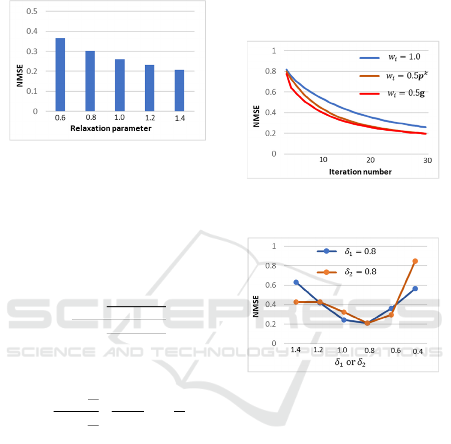
Figure 12: Plots of normalized mean square error versus
relaxation parameter. 200 detectors / view. 200 views.
Initial image is a uniform image of 1.0. Relaxation
parameter is changed from 0.6 to 1.4. 30 iterations.
3.4 Weighting Factors
To confirm the effect of the weight 𝑤
in eq. (8), we
introduce the new weighting factor, such that,
𝑤
=𝜇p
+𝜈g +𝛿,
(14)
where 𝜇,𝜈 and 𝛿 are in ℝ
respectively. From eqs.
(8) and (14), we obtain
f
=f
∑
𝑎
g
𝜇p
+𝜈g +𝛿
∑
𝑎
𝑝
𝜇p
+𝜈g +𝛿
.
(15)
If the weighting factor are set as 𝑤
=𝑝
, i.e. 𝜇=
1,𝜈=0,𝛿=0 , then the well-known ML-EM
algorithm is obtain, that is,
f
=f
∑
𝑎
g
p
∑
𝑎
𝑝
p
=
f
∑
𝑎
𝑎
g
𝑝
.
(16)
In this case 𝑎
is the probability that a positron
emitted from voxel j results in an event being
registered in sinogram bin i. If the weighting factor
are set as 𝑤
=1, i.e. 𝜇=0,𝜈=0,𝛿=1, then
standard ISRA is obtained.
Figure 13 illustrates the plots of the normalized
mean square error versus iteration number. We
computed three cases in eq. (15) and set the number
of detectors per view 200, the number of views per
360
∘
200, and the relaxation parameter the unit.
Initial data is a uniform image of 1.0, 1.0=f
∈ℝ
.
The blue line is NMSE at 𝜇=0,𝜈=0,𝛿=1, that is,
𝑤
=1.0. The orange line is at 𝜇=0.5,𝜈=0,𝛿=0,
that is, 𝑤
=0.5×𝒑
. The red line is at 𝜇=0,𝜈=
0.5,𝛿=0, that is, 𝑤
=0.5×g. From Fig. 13 we
can see that the method which have some weighting
factors are slightly better than standard ISRA.
Changing the range of μ from 2.0 to 0.05, there was
no influence in NMSE.
Figure 13: Plots of normalized mean square error versus
iteration number. 200 detectors/view. 200 views/2π. Initial
image is a uniform image of 1.0. Relaxation parameter is
the unit. The weight is changed.
Figure 14: Plot of the normalized mean square error versus
δ. 200 detectors/view. 200 views/2π. Initial image is a
uniform image of 1.0. Relaxation parameter is 1.4.
Figure 14 illustrates the plots of the normalized mean
square error versus 𝛿
and 𝛿
. The blue line is NMSE
in 𝛿
∈
1.4,0.4
if 𝛿
was fixed at 0.8. The orange
line is NMSE in 𝛿
∈
1.4,0.4
if 𝛿
was fixed at 0.8.
From Fig. 14 we can see that NMSE is the smallest if
both 𝛿
and 𝛿
was fixed at 0.8.
3.5 Noise Effects
To confirm the effect of the noise, gaussian noises are
added to the projection data. Using vector notation, it
can be expressed by
𝐠=A𝐟 + 𝐪,
(17)
where q indicates noise and is a normally distributed
deviate with zero mean and unit variance (Press et al.,
1992). To measure the effect of noise on the
reconstruction images, we use the signal-to-noise
Numerical Evaluation of the Image Space Reconstruction Algorithm
83
ratio (SNR) (Trussel, 2008). This is usually defined
as the ratio of signal power 𝜎
, to noise power 𝜎
,
SNR=
𝜎
𝜎
,
(18)
and in decibels
SNR
dB
=10×log
𝜎
𝜎
.
(19)
In projection data, the function power is usually
estimated by the simple summation
𝜎
=
1
𝑁
g
−𝜇
,
(20)
where 𝜇
is the mean of the projection data.
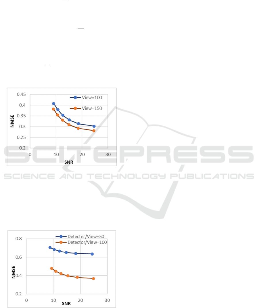
Figure 15: Plot of the normalized mean square error versus
SNR. 200 detectors/view. Initial data is a uniform image of
1.0. Iteration number is 30. The number of views/2π are
changed from 100 to 150.
Figure 15 illustrates the plots of the normalized mean
square error versus SNR. From Fig. 15 we can see that
the error decreases with increasing SNR and the error
decreases with increasing the number of views.
Figure 16: Plot of the normalized mean square error versus
SNR. 150 views/2π. Initial data is a uniform image of 1.0.
Iteration number is 30. The number of detectors/view are
changed from 50 to 100.
Figure 16 illustrates the plots of the normalized
mean square error versus SNR. From Fig. 16 we can
see that the error decreases with increasing SNR and
the error decreases with increasing the number of
detectors/view.
4 CONCLUSIONS
By discretizing the image reconstruction problem, we
applied ISRA to the problem and evaluated the image
quality. We showed that the error decreases with
increasing the number of detectors, views and
iterations. Also, we showed the effect of the
relaxation parameter and noise to the reconstructed
image.
We confirmed that the number of views,
detectors-source pair, relaxation parameters, iteration
numbers and weighting factors influenced the quality
of the reconstructed image. The size of system
matrices which were defined by detectors and views
was changed. If the size and iteration number was
large, computation of our algorithm consumed time
to large quantities. It is necessary to reveal the
optimal parameter of relaxation. By modifying the
weighting factors for the method of steepest descent,
it is possible to produce the new update methods. It is
important to evaluate the new methods.
REFERENCES
Herman, G. (2009). Fundamentals of Computerized
Tomography, 2
nd
edition, Springer-Verlag London.
Kak, A., Slaney, M. (1988). Principles of computerized
tomographic imaging, IEEE Press, New York.
Imiya, A. (1985) A direct method of three-dimensional
image reconstruction form incomplete projection, Dr.
Thesis, Tokyo Institute of Technology, Tokyo.
[Japanese]
Bendriem, B., Townsend, D. (1998). The theory and
practice of 3D PET, Kluwer Academic Publishers,
Dordrecht.
Stark, H. (1987). Image Recovery: theory and application,
Academic Press, New York.
Natterer, F., Wubbeling, F. (2001). Mathematical Methods
in Image Reconstruction, SIAM, Philadelphia.
Daniel, G. (2021) A new interpretation of (Tikhonov)
regularization, Inverse Problems, 37(6), 064002.
Ronny, R., Lothar R. (2019) Error estimates for Arnoldi–
Tikhonov regularization for ill-posed operator
equations, Inverse Problems, 35, 055002.
Simon, H., Ronny, R., Lukas W. (2022) On regularization
via frame decompositions with applications in
tomography, Inverse Problems, 38, 055003.
PHOTOPTICS 2024 - 12th International Conference on Photonics, Optics and Laser Technology
84

Depierro, A. (1987). On the convergence of the iterative
image space reconstruction algorithm for volume ECT,
IEEE trans. Med. Imaging, 6(2), 174-175.
Iniyatharasi, P., Pallikonda, M., Arun, T., Kannan, S.
(2015) PET image reconstruction using ISRA
technique, Australian J. Basic and Applied Sciences,
9(16), 110-117.
Depierro, A. (1993) On the relation between the ISRA and
the EM algorithm for positron emission tomography,
IEEE trans. Med. Imaging, 12(2), 328-333.
Reader, A., Letourneau, E., Verhaeghe, J. (2011)
Generalization of the image space reconstruction
algorithm, IEEE Nucl. Sci. Symp. Conf. Record. 4233-
4238.
Bertero, M., Mol, C., Pike, E. (1985), Linear inverse
problems with discrete data. I: general formulation and
singular system analysis, Inverse Problems, 1, 301-330.
Bertero, M., Mol, C., Pike, E. (1988), Linear inverse
problems with discrete data: II: stability and
regularization, Inverse Problems, 4, 573-594.
Luenberger, D. (1969). Optimization by vector space
methods, John Wiley & Sons. New York.
Luenberger, D. (2003). Linear and nonlinear programming,
Kluwer Academic Publishers. Boston, 2
nd
edition.
Censor, Y., Elfving, T., Herman, G., Nikazad, T. (2008).
On diagonally-relaxed orthogonal projection methods.
SIAM J. Sci. Comput. 30, 473-504.
Press, W., Teukolsky, S., Vetterling, W., Flannery, B.
(1992). Numerical Recipes in C, Cambridge University
Press. Cambridge, 2
nd
edition.
Aoyagi, T., Ohtsubo, K., Aoyagi, N. (2020)
Implementation and numerical evaluation for
multiplicative algebraic reconstruction techniques,
OPTICS & PHOTONICS International Congress
2020(The 6th Biomedical Imaging and Sensing
Conference).
Trussel, H., Vrhel, M. (2008). Fundamentals of Digital
Imaging, Cambridge University Press. Cambridge.
Numerical Evaluation of the Image Space Reconstruction Algorithm
85
