Learning Occlusions in Robotic Systems: How to Prevent Robots from

Hiding Themselves

Jakob Nazarenus

1 a

, Simon Reichhuber

2 b

, Manuel Amersdorfer

3 c

, Lukas Elsner

4 d

Reinhard Koch

1 e

, Sven Tomforde

2 f

and Hossam Abbas

4 g

Multimedia Information Processing Group, Kiel University, Hermann-Rodewald-Str. 3, 24118 Kiel, Germany

Intelligent Systems, Kiel University, Germany, Hermann-Rodewald-Str. 3, 24118 Kiel, Germany

Digital Process Engineering Group, Karlsruhe Institute of Technology, Hertzstr. 16, 76187 Karlsruhe, Germany

Chair of Automation and Control, Kiel University, Kaiserstr. 2, 24143 Kiel, Germany

Keywords:

Vision and Perception, Robot and Multi-Robot Systems, Simulation, Neural Networks, Classiﬁcation,

Autonomous Systems.

Abstract:

In many applications, robotic systems are monitored via camera systems. This helps with monitoring auto-

mated production processes, anomaly detection, and the reﬁnement of the estimated robot’s pose via optical

tracking systems. While providing high precision and ﬂexibility, the main limitation of such systems is their

line-of-sight constraint. In this paper, we propose a lightweight solution for automatically learning this oc-

cluded space to provide continuously observable robot trajectories. This is achieved by an initial autonomous

calibration procedure and subsequent training of a simple neural network. During operation, this network pro-

vides a prediction of the visibility status with a balanced accuracy of 90% as well as a gradient that leads the

robot to a more well-observed area. The prediction and gradient computations run with sub-ms latency and

allow for modular integration into existing dynamic trajectory-planning algorithms to ensure high visibility of

the desired target.

1 INTRODUCTION

With increasing computing capability, it is possi-

ble to make robotic systems more and more intelli-

gent. This includes improved perception of the en-

vironment and the robotic state so that an appropri-

ate action can be calculated based on this. Exam-

ples such as Boston Dynamics

show that robots can

solve path-ﬁnding problems even in unfamiliar terrain

in a similar way to animals and can hardly be dis-

tinguished from real animals in their movement se-

quences (Guizzo, 2019). The issue of localization of

robotic systems, especially multi-joint robotic arms,

https://orcid.org/0000-0002-6800-2462

https://orcid.org/0000-0001-8951-8962

https://orcid.org/0000-0002-6416-3453

https://orcid.org/0009-0001-8097-2373

https://orcid.org/0000-0003-4398-1569

https://orcid.org/0000-0002-5825-8915

https://orcid.org/0000-0002-5264-5906

https://bostondynamics.com/ (accessed January 29,

2024)

is challenging for robotics and sensor technology.

Various approaches directly place sensors on board to

detect the near proximity around the moving manip-

ulator and use known structures of the environment

for localization (Fan et al., 2021). Because of the

speed that can be achieved at the end of the arm, sen-

sors must provide high frame rates by simultaneously

lowering the resolution for real-time processing. In

contrast to the on-board approach, external, stationary

cameras exploit well-known reference positions en-

abling highly accurate positioning of moving objects

equipped with optical reference markers (Liu et al.,

2020). Besides the local restriction within the range

of the camera system, there is another crucial draw-

back in such systems, namely the line-of-sight occlu-

sions. With the term line-of-sight occlusion or sim-

ply occlusion we describe points within the viewing

cone of a camera where the direct line of sight to the

camera is interrupted by an obstacle, which means the

obstacle itself also counts as part of the occlusion (cf.

Figure 1). In the simple case, we have the exact posi-

tion of the robot and the environment, which allows us

482

Nazarenus, J., Reichhuber, S., Amersdorfer, M., Elsner, L., Koch, R., Tomforde, S. and Abbas, H.

Learning Occlusions in Robotic Systems: How to Prevent Robots from Hiding Themselves.

DOI: 10.5220/0012431000003636

Paper published under CC license (CC BY-NC-ND 4.0)

In Proceedings of the 16th International Conference on Agents and Artiﬁcial Intelligence (ICAART 2024) - Volume 2, pages 482-492

ISBN: 978-989-758-680-4; ISSN: 2184-433X

Occlusion

Visibility

Obstacle

Camera

Figure 1: Terminology line-of-sight occlusion.

to calculate the occlusion geometrically. However, it

is possible that the surroundings are unknown or that

the robot obscures itself. Especially in applications

where robotic arm movements are tracked by optical

markers, there is not only an interruption of the line-

of-sight when an external object interferes but also

self-occlusions occur at certain joint conﬁgurations.

When the reference point on the robot is occluded,

the pose estimation falls back to the imprecise for-

ward kinematics of the robot causing severe accuracy

issues.

To anticipate and prevent occluded states, we sug-

gest to construct a binary map of occluded robot states

given by a learned approximation, which can be used

for the trajectory calculation. The latter requires train-

ing data that represents the robot state space and its

occlusions fully sampling the possible robot states.

For this purpose, we provide a sampling routine that

can be used to provide data to model the occlusions.

At the end, we discuss the possibility of using the

occlusion model to reﬁne path planning by mini-

mizing the duration of occluded optical references.

For demonstration, we provide a showcase where a

robotic arm holds its end position statically while si-

multaneously moving the rest of the arm to reduce the

occlusions.

The remainder of the paper is structured as fol-

lows: The subsequent Section 2 lists the current state

of the literature about occlusions and robotic arm lo-

calization. Section 3 is divided into three parts: First,

we introduce the problem of learning occlusions as a

binary classiﬁcation problem and discuss the method-

ology of how to generate trajectories for the training,

second, we describe simulation methods and the real-

world experimental setup, and third, we introduce the

deep learning model for classiﬁcation. Afterward, in

Section 4, we present all results visually and discuss

them in Section 5. Finally, in Section 6, we conclude

the work and point out some further ideas for future

work.

2 RELATED WORK

The issue of detecting occlusions of important areas

that occur when recording robotic systems with static

camera systems is highly task-dependent. It is often

more appropriate to use a moving camera (Silva and

Santos-Victor, 2001) and to analyze the occlusion us-

ing different perspectives. An explicit detection of

occlusion in a stream-based fashion based on optical

ﬂows has already been shown (Ayvaci et al., 2012).

Here, the obstacle or the camera is moving, which

simpliﬁes the detection of obstacles, since the line-of-

sight between both is temporally given. However, this

method is not applicable to static obstacles. Besides

explicit detection of occlusions, there are two implicit

methods of how to cope with them. First, the addi-

tion of stationary-placed sensors allows looking be-

hind the occlusion. Instead of learning the spatial dis-

tribution of blind spots, some approaches try to reveal

blind spots by merging other more pervasive sensors

with the occluded sensor. A common way is the us-

age of Radio-Frequency sensors, which enable local-

ization with centimeter-scale precision (Boroushaki

et al., 2021). A radio-frequency perception is able

to penetrate non-conducting materials enabling the

tracking of an external Radio-Frequency Identiﬁca-

tion (RFID) reference.

Second, onboard sensors can measure the near

proximity of all moving parts of the robot which turns

the environment into the state of reference and obvi-

ously eliminates the line-of-sight from the reference

(environment) to the robot. When certain known ob-

jects in the environment are detected, a relative lo-

calization is allowed. Knowing only the type and

shape of the object, the robot is able to interact in-

place with the object. Otherwise, if only the distance

to collision is measured only collision avoidance is

possible. Directly tracking the object of observation

and its near proximity by onboard sensors is another

way to prevent occlusions and collisions. For ex-

ample, the tracking of human arm motions using an

Inertial Measurement Unit (IMU) and potentiometer

has been proposed (Shintemirov et al., 2020). As a

ground truth to evaluate the localization accuracy of

a capsule equipped with IMU and a camera system

for endoscopy, Vedaei and Wahid placed the capsule

on a robotic arm and tested movements that naturally

occur gastrointestinally (Vedaei and Wahid, 2021).

Another onboard sensor approach is proximity

sensing (Gandhi and Cervera, 2003), which has been

shown in (Fan et al., 2021) using surface waves. Be-

sides this external sensors are used to track the robotic

system or parts that it interacts with, e.g. part local-

ization in grasping applications (Zheng et al., 2018).

Learning Occlusions in Robotic Systems: How to Prevent Robots from Hiding Themselves

483

To lower the complexity of occlusions, for some

tasks, it is appropriate to model them in only two di-

mensions. For example, given the task of mechan-

ical search, where a manipulator has to ﬁnd objects

that are occluded by other ones, the occlusions can

be visualized by a 2-dimensional heat map (Daniel-

czuk et al., 2020). In the following, we use the term

occlusion as an abbreviation for interruptions in the

line-of-sight of a camera to the optical reference point

at the robot end effector. The occlusions are there-

fore camera-speciﬁc. Enriching the joint space of the

robot with the binary information about the line-of-

sight of a camera allows the planning of trajectories

that minimize the duration of line-of-sight interrup-

tion between the camera and the end effectors.

3 METHODS

The visibility of a point at an n-Degrees of Freedom

(DoF) robot can be modeled by a function f : R

→

{0,1} that takes the joint angles of the robot as an in-

put and has a binary output with 1 representing the

visible, and 0 representing the hidden state. The par-

tial visibility of a non-point-like extended object can

be expressed by loosening the function deﬁnition to

allow mapping to values in the interval [0, 1]. This

function is highly complex as it depends on the pose

of the camera, the geometry of the robotic system and

its surroundings, as well as its kinematics. Our ap-

proach is to learn this function in a supervised manner

by automatically sampling the domain of the function

and observing the corresponding output. We then use

these samples to employ efﬁcient data-driven meth-

ods to ﬁnd an estimate for f . To evaluate the capa-

bilities of the employed methods, we used the Bal-

anced Accuracy (bAcc), e. g. found in (Brodersen

et al., 2010). For a set of matched inputs, it is given as

the arithmetic mean of Sensitivity (SEN) and Speci-

ﬁcity (SPEC)

bACC =

(SEN + SPC) =



T P

T N



. (1)

Here, TP (TN) is the number of correctly posi-

tively (negatively) classiﬁed samples, while P and N

are the number of positive and negative samples. The

balanced accuracy is used here because the dataset

is highly imbalanced in favor of the visible samples.

Similarly to the F1 score (Rijsbergen, 1979), the bAcc

is used in such situations to create a more balanced

measure for the problem. We chose the balanced ac-

curacy as it is easily interpretable and in comparison

to the F1 score does not put more emphasis on the

positive class.

3.1 Trajectory Generation

For the supervised training of our occlusion predic-

tion model, we need to obtain a set of points in the

state space of the robot with their corresponding oc-

clusion status. This training set needs to be large

enough to allow learning-based models to generalize

their knowledge for independently sampled test data.

As a simple strategy, a set of points is uniformly sam-

pled from the state space Q ⊆ R

for a robot with n

joints. While this approach might work well with sim-

ulated robots, it does not provide a traversable path

for real robots due to violating the velocity and ac-

celeration constraints. Therefore, an automatic gen-

eration of training trajectories is required. In this

section, we describe a method to generate a continu-

ous path closely resembling the uniform sampling ap-

proach under the given kinematic constraints. Fourier

series are commonly used to design excitation trajec-

tories for parameter identiﬁcation in robotics (Swev-

ers et al., 1997b; Swevers et al., 1997a; Park, 2006;

urz et al., 2017). We utilize the concept in the form

of smooth random functions (Filip et al., 2019). Here,

the trajectory of each joint i ∈ {1, ..., n} is deﬁned as

(t) =

∑

k=0



i,k

cos



2πkt



+ b

i,k

sin



2πkt



(2)

with b

i,0

= 0, where a

i,k

and b

i,k

are the Fourier coef-

ﬁcients, m is the number of modes, and T denotes the

trajectory period. We normalize the generated func-

tion values to unit variance. In the following, we con-

sider the coefﬁcients a

i,k

and b

i,k

to be sampled from

N (0,1/(2m + 1). An alternative method of optimiz-

ing these coefﬁcients is shown in Appendix A. The

corresponding trajectory velocity ˙q

(t) and accelera-

tions ¨q

(t) are obtained directly from the Fourier se-

ries’ time derivatives. The trajectories have to satisfy

the kinematic and dynamic constraints of the robotic

manipulator. Let (q

i,min

i,max

) be the lower and up-

per bound for the angle of robot joint i. Its angu-

lar velocity and acceleration limits are denoted as

˙q

i,max

and ¨q

i,max

respectively. This leads to the state

space deﬁnition Q := {q ∈ R

i,min

≤ q

i,max

, i ∈

{1, ..., n}}.

An exemplary path for a single joint with m = 10

and T = 2 is shown in Figure 2. While for any t, its

function value is randomly distributed according to

N (0,1) under the random choice of the coefﬁcients

and b

(Filip et al., 2019), for a single path the dis-

tribution deviates from N (0,1) due to the individual

function values not being independent. This can be

seen in Figure 2, where the trajectory for m = 10 and

T = 2 is relatively smooth.

With increasing m, the random function becomes

ICAART 2024 - 16th International Conference on Agents and Artiﬁcial Intelligence

484

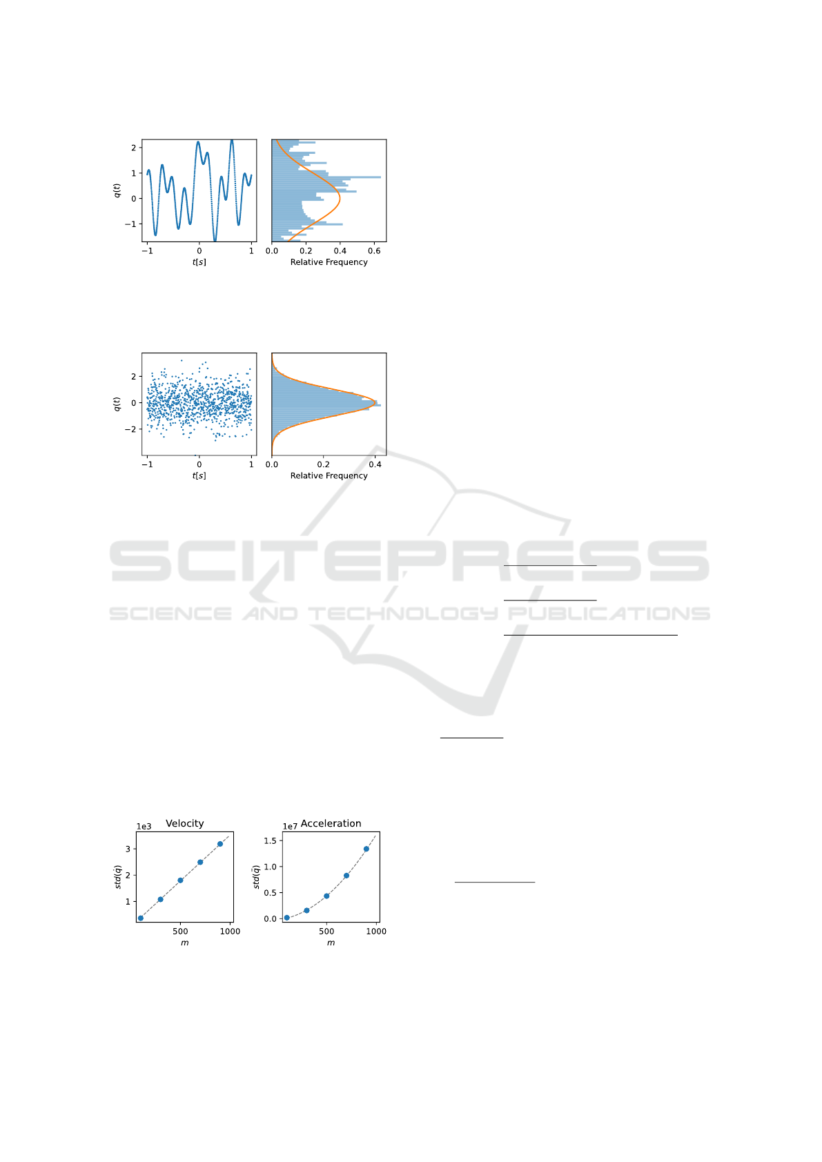
Figure 2: Smooth random path (left) with its spatial distri-

bution (right) for a mode count of m = 10. The orange line

shows the distribution for the limit of inﬁnite modes or inﬁ-

nite paths.

Figure 3: ”Smooth” random path (left) with its spatial dis-

tribution (right) for a mode count of m = 10

. The spatial

distribution approaches its limit of a Gaussian distribution.

less smooth and oscillates more often. This reduces

the dependency of successive function values and thus

the deviation from N (0,1). This behavior can be seen

in Figure 3 for m = 10

and T = 2.

While this randomness is desirable for the efﬁcient

sampling of the joint space, there are limits given by

the maximum angular speed and acceleration of the

robot. When observing the ﬁrst and second deriva-

tives, we see them increasing as shown in Figure

4. This prevents the arbitrary increase of the mode

count m, as it would inevitably cause violations of the

robot’s kinematic constraints. In our case, we want to

generate a path that maximizes the variability under

the given constraints for the function values and its

ﬁrst two derivatives. For this purpose, we propose the

following approach shown in Algorithm 1. For each

Figure 4: Increasing mode counts leads to higher velocities

and accelerations. The dashed line shows a linear ﬁt for the

velocity and a quadratic ﬁt for the acceleration.

joint, we initially ﬁnd the highest mode count m that

causes the ˙q and ¨q constraints to not be violated most

of the time. To achieve this, we choose a threshold

of 95% (2σ) of the data to be below the given lim-

its. Increasing this threshold causes fewer violations,

but at the same time reduces the reached mode count

m and thus the variability of the generated data. For

the generated trajectories, we enforce the ˙q and ¨q con-

straints by locally slowing down the time via the func-

tion localTimeScaling(). Then, any violations of

the angular constraints are removed by replacing the

violating parts of the trajectory with quadratic poly-

nomials via the function quadraticClipping(). As

both functions alter the overall duration of our tra-

jectory, we enclose this process with a search for the

optimal input duration and terminate once the search

interval falls below a predeﬁned threshold ∆T . This

threshold causes the resulting trajectories for all joints

to slightly differ in their duration, which necessitates

the artiﬁcial slowing of all but the longest generated

trajectory via the method alignToSlowest().

3.1.1 Local Time Scaling

With discretized time, the ﬁrst and second derivatives

are computed as

˙q

(t) =

(t + ∆t) − q

(t)

∆t

, (3)

¨q

(t) =

˙q

(t + ∆t) − ˙q

(t)

∆t

(t + 2∆t) − 2q

(t + ∆t) + q

(t)

∆t

Given a maximum angular velocity ˙q

i,max

and ac-

celeration ¨q

i,max

, if a velocity or acceleration limit

is exceeded, we can enforce it by scaling the time

locally. This is achieved by multiplying the time

with a factor ˙q

(t)/ ˙q

i,max

for velocity constraints and

¨q

(t)/ ¨q

i,max

for acceleration constraints. To avoid

unnecessary scaling of the whole path, we conﬁne

this scaling locally by only considering regions where

the constraint is violated. Given such a region with

a duration of t

, center t

, a maximum value of

˙q

max

) or ¨q

max

) respectively, the time scaling is

given by a Gaussian with mean t

and standard devia-

tion t

. This Gaussian is rescaled to have a minimum

value of 1 and a maximum value of ˙q

max

)/ ˙q

i,max

¨q

max

)/ ¨q

i,max

respectively. This reduces the ac-

celeration and velocity locally to stay within the given

bounds. The overall time scaling factor is then given

by the maximum of all Gaussians for a given time

step. Figure 5 shows an example of the time scaling

for velocity and acceleration constraints.

Learning Occlusions in Robotic Systems: How to Prevent Robots from Hiding Themselves

485

all

← [ ],[ ];

for i ∈ [1, n] do

initialize (T

min

max

);

while T

max

− T

min

> ∆T do

mean

← (T

max

+ T

min

)/2;

initialize (m

min

max

);

while m

max

− m

min

> 1 do

mean

← ⌊(m

max

+ m

min

)/2⌋;

Q ← smRanFun(T

mean

);

Q ← derivatives(Q);

if 2 ∗ std(

Q) < ˙q

i,max

& 2 ∗ std(

Q) <

¨q

i,max

then

min

← T

mean

;

else

max

← T

mean

;

end

T ← localTimeScaling(Q, T

mean

˙q

i,max

, ¨q

i,max

);

T ← quadraticClipping(

T , q

i,min

i,max

, ¨q

i,max

);

T < T then

min

← T

mean

;

else

max

← T

mean

;

end

all

.append(

Q);

all

.append(

T );

all

← alignToSlowest(Q

all

);

return Q

all

;

end

Algorithm 1: Automatic sampling trajectory genera-

tion based on smooth random functions. The abbre-

viated method smRanFun() describes the generation of

a smooth random function that is normalized according

to the given angular constraints.

3.1.2 Quadratic Clipping

To enforce the position constraints, we replace the

parts exceeding the angular constraint q

i,max

by a

quadratic function. The quadratic coefﬁcient is given

by the acceleration constraint ¨q

i,max

. However, not

only the exceeding points need to be replaced but also

points with an angular velocity so high that it is guar-

anteed that the angular constraint will be exceeded

due to the acceleration constraint. To determine these

points, for each time step t we compute the neces-

sary angular acceleration ¨q

i,stop

(t) > 0 to stop right at

i,max

. We denote the corresponding time as t

max

. In

the following considerations,

t > t denotes a time step

along the path of maximal deceleration. We compute

the required acceleration value as

Figure 5: Local time scaling enforces the constraints on the

ﬁrst and second derivatives of the signal. For better visibil-

ity, the time axis is kept the same for all plots. The clipped

gray line shows the original signal while the blue line shows

the modiﬁed signal. The lower ﬁgure shows the ratio by

which the time is locally delayed in order to constrain the

derivatives.

(

t) = q

(t) + ˙q

(t)

t −

¨q

i,stop

(t)

(4)

˙q

max

) = ˙q

(t) − ¨q

i,stop

(t)t

max

= 0

=⇒ t

max

˙q

(t)

¨q

i,stop

(t)

max

) = q

i,max

= q

(t) +

˙q

(t)

¨q

i,stop

(t)

−

˙q

(t)

2 ¨q

i,stop

(t)

=⇒ ¨q

i,stop

(t) =

˙q

(t)

2(q

i,max

− q

(t))

If ¨q

i,stop

(t) > ¨q

i,max

holds, we know that the po-

sition constraint will be exceeded even if maximum

deceleration is used to reduce the velocity. Thus, for

each of these regions, we ﬁnd the last valid time step

before this region and the ﬁrst valid time step t

af-

ter this region. We then compute a quadratic function

that starts at t

with initial velocity ˙q

) and constant

acceleration ¨q

i,stop

) and ends at t

max

with a velocity

of 0. Symmetrically, we compute a second quadratic

function that starts at t

with initial velocity ˙q

) and

constant acceleration ¨q

i,stop

) and continues back-

ward in time until it reaches q

i,max

with a velocity of

0. Both functions meet at q

i,max

. For enforcing min-

imum values, this method is applied to the inverted

input signal. Figure 6 demonstrates this method.

As shown in Figure 6, the early deceleration

causes a gap between the two quadratic functions.

ICAART 2024 - 16th International Conference on Agents and Artiﬁcial Intelligence

486

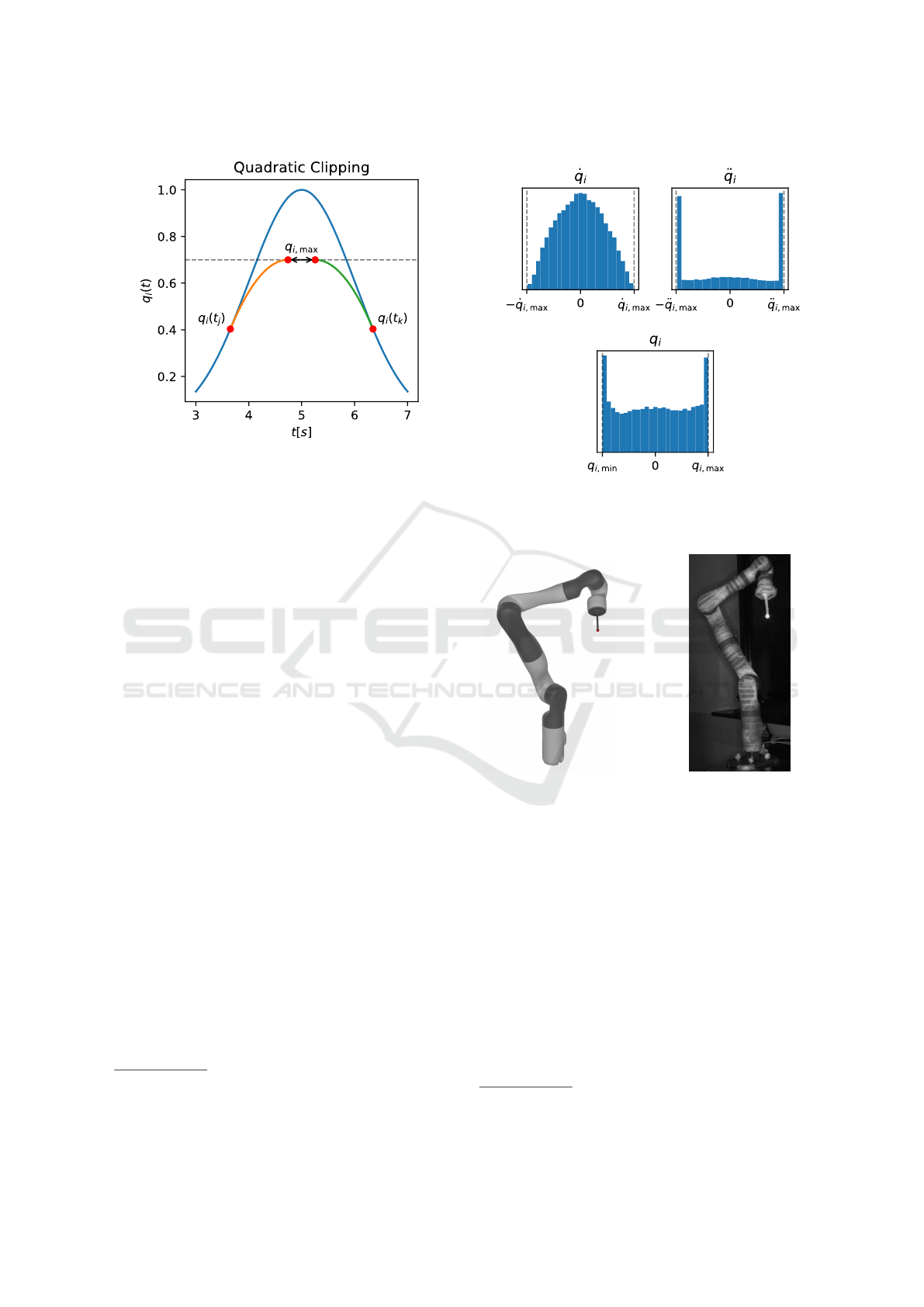
Figure 6: Clipping off out-of-range positions by replacing

with quadratic polynomials.

Closing this gap causes a slight reduction in overall

signal length. In combination with the artiﬁcial in-

crease in signal length by the local time scaling, this

necessitates the binary search for the optimal duration

as shown in Algorithm 1.

In summary, the proposed algorithm ﬁnds a

smooth random path for each joint that maximizes

the overall randomness under the given constraints

for the angles as well as angular velocity and accel-

eration. The distribution of a single generated trajec-

tory is shown in Figure 7. It is directly visible how

out-of-range values are shifted towards the limits of

the allowed range. For the angle q

, its distribution

thus resembles a uniform distribution with peaks at

its boundaries.

In Appendix A, we present an alternative ap-

proach to plan a feasible excitation trajectory by ob-

taining the Fourier coefﬁcients of (2) directly from a

nonlinear optimization problem.

3.2 Simulation

To test the feasibility of the approach, we created

an experiment in the open-source software Blender

The scene contains a single camera as well as a model

of the Kinova Gen2 7 DoF robot

that has a spherical

marker attached to the tip of the end-effector as a tar-

get, as seen in Figure 8a. The goal of our approach

is to ensure the visibility of this target under arbitrary

movements of the robot. Using the Blender Python

https://www.blender.org/ (accessed January 29, 2024)

https://github.com/Kinovarobotics/kinova-ros (ac-

cessed January 29, 2024)

Figure 7: Distribution of a trajectory generated by the pro-

posed path generation algorithm as well as the distribution

of its ﬁrst two derivatives.

(a) Simulation. (b) Laboratory Setup.

Figure 8: Simulated and real-world evaluation setups. The

simulation is based on the publicly available robot model of

the Kinova

Gen2 robotic arm.

API

, we implemented a script that reads a trajec-

tory and simulates the robot’s pose for each time step.

Then, we determined whether the marker was visible

or hidden. This is done via a single traced ray, so it

is not necessary to render the full scene, resulting in

a simulation rate of ≈ 5 · 10

steps per second. The

simpliﬁcation is necessary for efﬁcient sampling and

results in a discontinuous binary output. Furthermore,

it is possible to simulate any non-smooth trajectory,

such as randomly sampled joint angles. This allows

to create data for testing against the generated smooth

trajectories.

https://docs.blender.org/api/current/index.html (ac-

cessed January 29, 2024)

Learning Occlusions in Robotic Systems: How to Prevent Robots from Hiding Themselves

487

3.3 Real-World Setup

We built a setup very similar to the simulation in our

laboratory, with the same Kinova robot, and attached

a 3D printed version of the instrument with a small

reﬂective sphere at its tip representing the point of

interest as shown in Figure 8b. We then utilized a

camera (Qualisys Arqus A9) with its own light source

to automatically detect whether the marker is visible

or not. This is achieved using thresholding visible

marker size, resulting in a similar binary signal as in

the simulation case. To prevent unwanted reﬂections

on smooth surfaces of the robot, we covered it in not-

reﬂective tape. We determined the limits for each of

the robotic joints to prevent collisions during the au-

tomatic capturing process and generated a trajectory

with a duration of 6 h. The trajectory is executed by

the Kinova robot using its ROS interface. Therefore,

a PD controller is designed to track the position and

velocity reference of the trajectory sufﬁciently con-

sidering the actual joint position and velocity mea-

surements. The resulting velocity commands are then

commanded to the robot’s joint drives.

3.4 Classiﬁcation with Multilayer

Perceptrons (MLPs)

There are several Machine Learning (ML) algorithms

in the literature for supervised classiﬁcation that have

one or more disadvantages (Bishop and Nasrabadi,

2006; Cover and Hart, 1967; McNicholas, 2016;

Cortes and Vapnik, 1995; Sch

olkopf and Smola,

2005). Problems can arise from the complexity of the

model or the sensitivity of the hyperparameters. For

example, Nearest Neighbor models (Cover and Hart,

1967) require all training points to be stored, which is

not computationally feasible in our scenario. Other

ML models, like Support Vector Machines (Cortes

and Vapnik, 1995; Sch

olkopf and Smola, 2005))

or Gaussian Models for Classiﬁcation (McNicholas,

2016) use only a subset of the data. Unfortunately,

these models are highly dependent on hyperparam-

eters and also require high computational resources

when trained on raw data. In contrast to this, MLPs

have shown the ability to represent highly complex

functions (Hornik, 1991). With low layer counts the

computational requirements for training are low while

providing an efﬁcient representation of the sampled

space. For this reason, they are used in learning high-

dimensional spaces, such as 5-dimensional scene rep-

resentations for view synthesis in Neural Radiance

Fields (NeRFs) (Mildenhall et al., 2021). Further-

more, due to their widespread availability in machine-

learning frameworks, they are easily deployed with

hardware acceleration, thus beneﬁting from a high de-

gree of parallelization. Another crucial beneﬁt is that

it is computationally cheap to compute their gradi-

ent. This is necessary for integrating them as part of

a larger optimization problem in the context of trajec-

tory planning. One potential drawback of this method

is that MLPs are struggling to learn high-frequency

details. For the robot used in our scenario, this did not

pose any problems due to the simplicity of its geome-

try. However, for mesh-like structures with ﬁne detail,

an approach based on a positional encoding would be

beneﬁcial (Mildenhall et al., 2021).

In our case, the chosen network architecture starts

with an input layer with n inputs representing the

robot’s joint angles. A series of fully connected lay-

ers follows, each with a Rectiﬁed Linear Unit (ReLU)

activation function that we chose for their computa-

tional efﬁciency. Finally, a fully connected layer com-

bines the hidden layers’ activations and passes them

through a ﬁnal single sigmoid activation function to

map the ﬁnal output to the interval [0,1]. For opti-

mization, we chose the Adam optimizer (Kingma and

Ba, 2014). All hyperparameters were determined via

hyperparameter optimization using the Asynchronous

Successive Halving Algorithm (ASHA) scheduler (Li

et al., 2020) and the Optuna search algorithm (Akiba

et al., 2019). As a loss function we used binary cross-

entropy, which is a commonly used loss for binary

classiﬁcation problems

L(Y

pred

true

) =

∑

i=1

−α

[ Y

true

logY

pred

(5)



1 −Y

true



log



1 −Y

pred



The balancing factor α

is used to increase the con-

tribution of underrepresented samples. With P being

the number of positive samples and N being the num-

ber of negative samples, the factor is set to

P+N

for

positive and to

P+N

for negative samples.

During the training, 20% of the data were used

as validation data. The validation and training data

are chosen as continuous parts of the trajectory, as

random shufﬂing would with a high likelihood cause

close training samples for every validation sample. To

further reduce this risk, a buffer between the two seg-

ments with a length of 1% of the data was removed

before training. Besides this evaluation data, for the

simulated scenario, we created a test set of 10

uni-

formly sampled robot conﬁgurations to avoid overﬁt-

ting on the validation data. All models were imple-

mented in the PyTorch framework and trained on a

consumer-level system with a Ryzen 3600 as a CPU,

a GTX 1660 Ti as a GPU, and 16 GB of Memory. We

ICAART 2024 - 16th International Conference on Agents and Artiﬁcial Intelligence

488

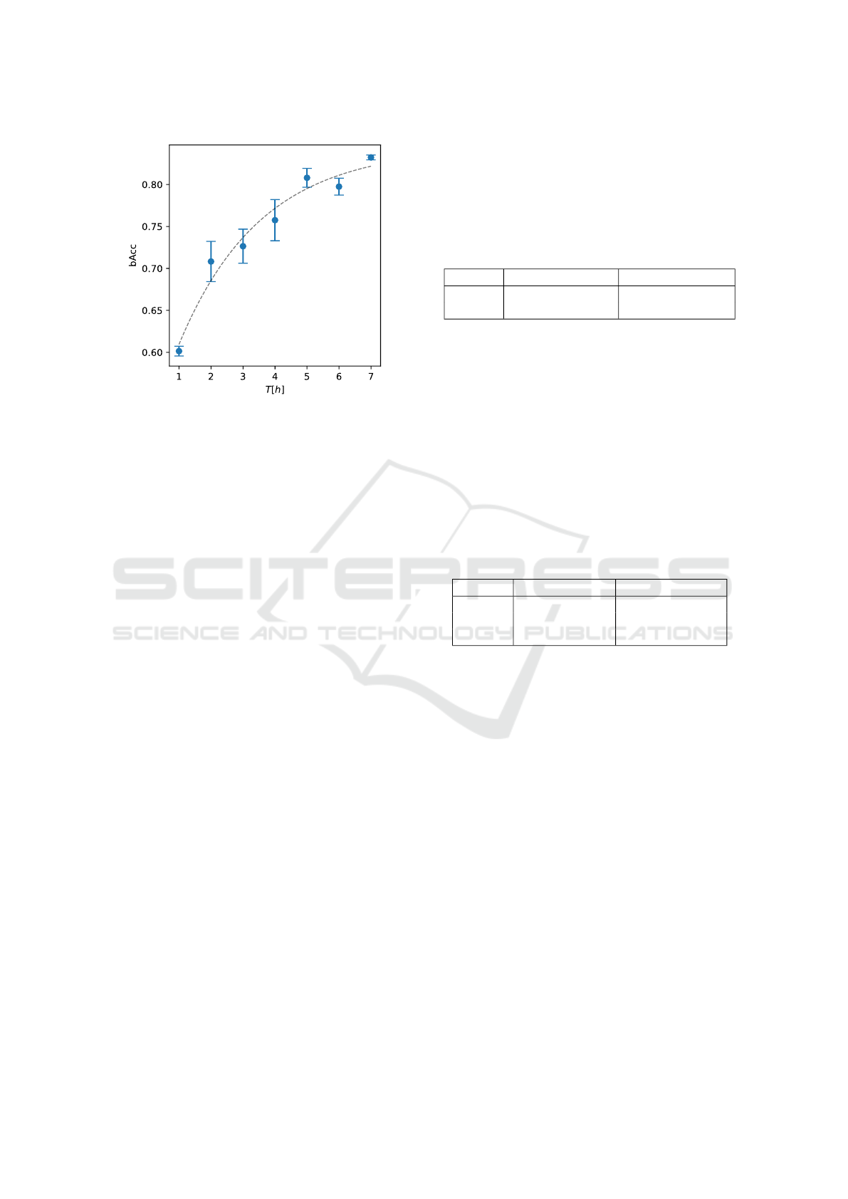
Figure 9: bAcc scores were measured on the test set for in-

creasing trajectory durations. For better visualization, the

dashed line shows a ﬁt for an exponentially decaying func-

tion.

trained for 5 · 10

epochs but stopped early if no im-

provement was seen in the validation score for 10

epochs. In these conditions, training a single network

takes approximately 1 min.

4 RESULTS

In this section, we show the training results for the

MLPs with a focus on the required trajectory length,

the hyperparameter tuning, and computational efﬁ-

ciency. Furthermore, we demonstrate with a short ex-

ample how the MLP can be integrated into trajectory-

planning to increase the overall visibility.

We initially established a baseline score by train-

ing on a simulated dataset of 10

uniformly sampled

joint states. When trained until saturation, the net-

work scored a balanced accuracy of 94% for predict-

ing the correct visibility of the chosen target.

For smooth simulated trajectories, the results

show increasing test scores as shown in Figure 9. Af-

ter a steep increase at the beginning, the increase in

gained balanced accuracy reduces at higher durations.

Due to these diminishing returns, we chose six hours

as the duration for all further experiments.

For a simulated trajectory with a duration of six

hours, the hyperparameter optimization yielded the

following results

• learning rate: 2 · 10

−3

• number of hidden layers: 2,

• size of hidden layers: 78.

With these parameters, when trained until satu-

ration on a simulated trajectory of 6 h, the model

achieves a balanced accuracy of 85% on the uni-

formly sampled test set. A more detailed view of this

result is shown by the confusion matrix in Table 1.

Based on these results, the recall for the visible class

Table 1: Confusion matrix for the predictions of the MLP

trained on a rendered 6 h smooth trajectory. The values are

normalized by the total number of samples in the test set.

Predicted Visible Predicted Hidden

Visible 74.28% 12.34%

Hidden 2.07% 11.30%

is 85.75% and 84.53% for the hidden class. Further-

more, the overall ratio of visible samples in the dataset

is 86.63%. The measured precision is 97.29% for the

visible and 47.80% for the hidden class.

To conﬁrm these simulation results, we captured

the same 6 h trajectory on our real-world setup (see

Figure 8b) and trained the MLP on this data until

no further improvement was noticed. We obtained

slightly higher bAcc scores of 90% in this case.

When evaluating the model’s latency on 1 · 10

samples, we found the results shown in Table 2. Fur-

thermore, every measured latency stayed below 1 ms.

Table 2: Inference and gradient computation times for the

proposed MLP.

Forward-Pass Backward-Pass

mean 78 µs 391 µs

5% low 95 µs 478 µs

1% low 150 µs 626 µs

To show the feasibility of the proposed approach,

we chose a simple test case: Increasing the visi-

bility under the constraint of a stable end-effector.

We modeled this via the forward kinematics function

e(Q) : R

→ R

, that provides the position of the end-

effector for a given combination of joint angles Q.

Furthermore, the trained MLP is denoted as the func-

tion v(Q) that predicts the visibility of the robot at

a given state. For a starting conﬁguration Q

start

ﬁnd a trajectory that maximizes the visibility under

the constraint of a stable end-effector by reducing the

following loss

L(Q) = γ

||e(Q) − e(Q

start

)|| + γ

(1 − v(Q)). (6)

The ﬁrst part of this loss reduces deviations in the end-

effector position from the initial conﬁguration while

the second part increases the overall visibility using

the trained MLP. The weight factors γ

and γ

allow

us to put more emphasis on one of the two aspects

during optimization. In our case, we chose γ

= 10

and γ

= 1 to ensure a stable end-effector position.

The trajectory is then obtained by repeated com-

putations of the gradient ∇

and changing Q in the

Learning Occlusions in Robotic Systems: How to Prevent Robots from Hiding Themselves

489

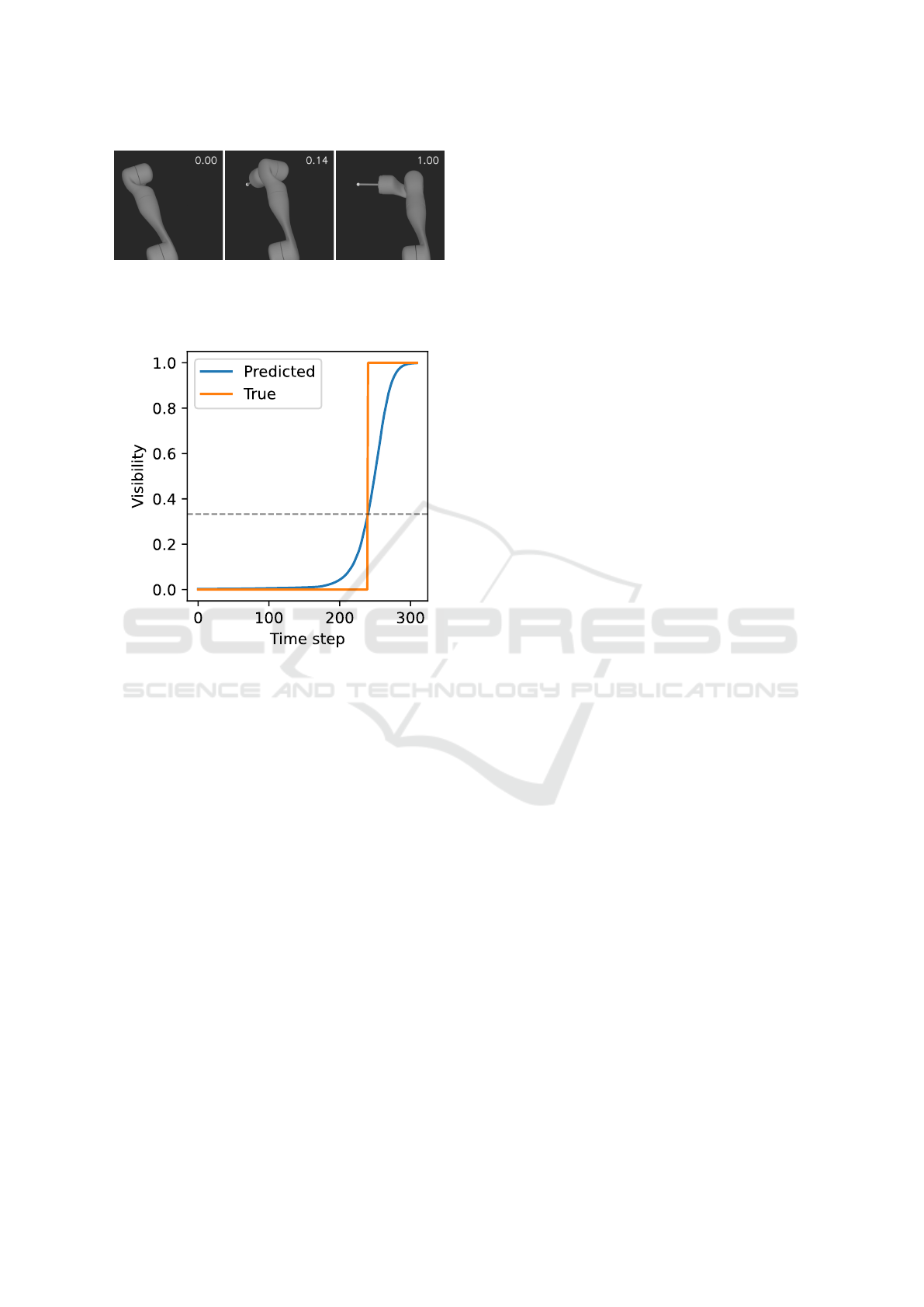
Figure 10: Renderings of a trajectory that maximizes the

visibility of the target at the end-effector (bright sphere)

while keeping it stable. The corresponding predicted vis-

ibility scores are shown in the upper right.

Figure 11: Predicted and rendered visibility along the gen-

erated trajectory.

opposite direction of this gradient. The generated

trajectory is shown qualitatively in Figure 10. As

shown in Figure 11, the predicted visibility increases

smoothly and corresponds to the measured visibility.

The object becomes visible at a predicted visibility

value of 0.33.

5 DISCUSSION

As shown by the 94% bAcc score on the synthetic uni-

formly sampled dataset, MLPs are a valid choice for

learning the complex occlusion behavior of robotic

systems. This score serves as a benchmark for smooth

random functions. As Figure 9 shows, the added vari-

ability in the data from an increased trajectory dura-

tion beneﬁts the training results. However, even con-

sidering MLPs trained on 6 h trajectories with ﬁne-

tuned hyperparameters, there is still a difference of 9

percentage points in the bAcc score. This shows that

even though the smooth random functions slowly ap-

proach the benchmark score, this method of sampling

does not fully reach the desired score at durations that

are feasible to run in real-world applications. When

investigating the results further, we found that the re-

call predicting either the visible or the hidden class

was close to the measured bAcc of 85%, however,

their respective recall is much higher for the visi-

ble class. This can largely be attributed to the high

class imbalance in our dataset, which highly favors

the visible class with 86.63%. The re-balancing fac-

tors caused by this imbalance drastically increase the

contribution of the hidden class to the overall loss,

which leads to the relatively high number of samples

falsely classiﬁed as hidden.

One major limitation of our sampling method is

that there is no feedback from the measured visibil-

ity to the sampling routine. This has the advantage

that it allows for both components to run on separate

hardware without the need for a real-time intercon-

nection. While the separation of surveillance and con-

trol systems might represent reality in many scenar-

ios, there are possibly important performance gains

to be found without this limitation. Furthermore, such

an approach would remove the need for synchroniza-

tion between the two systems.

Another limitation of the proposed method is its

reliance on a stationary camera. The MLP’s approxi-

mated function depends highly on the camera’s pose,

moving the camera requires retraining the model. At

the same time, the model generally does not depend

on the camera’s intrinsic. For this reason, changes in

distortion or focal length do not require resampling

and retraining the model.

An interesting ﬁnding is that the model’s perfor-

mance seems to be slightly higher on the real-world

data than on the rendered training data. This could

possibly be attributed to the small differences between

the real and the simulated scene. One of the param-

eters that could have inﬂuenced this difference is the

positioning of the camera, which differs between sim-

ulation and reality (see Figure 8).

Finally, we could show that the proposed method

of using MLPs is computationally efﬁcient enough

for the application in real-time trajectory planning al-

gorithms. Inference and gradient computation in the

sub-ms latency range allows for real-time prediction

and optimization. As we have shown in the example

application, the trained MLP is easily integrated into

trajectory planning and allows for the continuous op-

timization of the robot’s observability under chosen

constraints.

ICAART 2024 - 16th International Conference on Agents and Artiﬁcial Intelligence

490

6 CONCLUSION AND OUTLOOK

In this paper, we proposed a method for automatically

improving the visual observability of robotic systems.

This method relies heavily on our two main contri-

butions, the automatic sampling of the training space

via modiﬁed smooth random functions as well as the

training and evaluation of lightweight MLPs to repre-

sent the occlusion function. While there is still room

for improvement due to the measured performance

gap between independently sampled data and smooth

trajectories, we could show that this approach works

well in the simulation and real-world experiments and

consistently shows high validation scores. We fur-

ther showed the modular integration in a trajectory-

planning example, where it successfully increased the

visibility under given constraints.

There are several directions for further research,

the most promising being a smart coupling of the tra-

jectory generation with live feedback from the camera

system. This would potentially allow for more efﬁ-

cient approaches to sampling the boundary between

visible and hidden states, thus reducing the dimen-

sionality of the problem. Another promising approach

would be to disentangle camera pose, robot geometry,

and robot kinematics into several learned components

of a combined system. This would possibly allow it to

be more resilient against minor changes in the scene

and would only require minor retraining upon repo-

sitioning the camera. Another research direction is

investigating different robot geometries and material

properties. This could include semi-translucent and

reﬂective surfaces as well as the addition of positional

encodings for handling more complex joint geome-

tries.

ACKNOWLEDGEMENT

This research is funded through the Project ”OP

der Zukunft” within the funding program by

Europ

aischen Fonds f

ur Regionale Entwicklung

(REACT-EU).

REFERENCES

Akiba, T., Sano, S., Yanase, T., Ohta, T., and Koyama, M.

(2019). Optuna: A next-generation hyperparameter

optimization framework. In Proceedings of the 25th

ACM SIGKDD International Conference on Knowl-

edge Discovery and Data Mining.

Ayvaci, A., Raptis, M., and Soatto, S. (2012). Sparse occlu-

sion detection with optical ﬂow. International journal

of computer vision, 97:322–338.

Bishop, C. M. and Nasrabadi, N. M. (2006). Pattern recog-

nition and machine learning, volume 4. Springer.

Boroushaki, T., Leng, J., Clester, I., Rodriguez, A., and

Adib, F. (2021). Robotic grasping of fully-occluded

objects using rf perception. In 2021 IEEE Inter-

national Conference on Robotics and Automation

(ICRA), pages 923–929. IEEE.

Brodersen, K. H., Ong, C. S., Stephan, K. E., and Buhmann,

J. M. (2010). The balanced accuracy and its posterior

distribution. In 2010 20th international conference on

pattern recognition, pages 3121–3124. IEEE.

Cortes, C. and Vapnik, V. (1995). Support-vector networks.

Machine learning, 20:273–297.

Cover, T. and Hart, P. (1967). Nearest neighbor pattern clas-

siﬁcation. IEEE transactions on information theory,

13(1):21–27.

Danielczuk, M., Angelova, A., Vanhoucke, V., and Gold-

berg, K. (2020). X-ray: Mechanical search for an oc-

cluded object by minimizing support of learned occu-

pancy distributions. In 2020 IEEE/RSJ International

Conference on Intelligent Robots and Systems (IROS),

pages 9577–9584. IEEE.

Fan, X., Simmons-Edler, R., Lee, D., Jackel, L., Howard,

R., and Lee, D. (2021). Aurasense: Robot colli-

sion avoidance by full surface proximity detection. In

2021 IEEE/RSJ International Conference on Intelli-

gent Robots and Systems (IROS), pages 1763–1770.

IEEE.

Filip, S., Javeed, A., and Trefethen, L. N. (2019). Smooth

random functions, random odes, and gaussian pro-

cesses. SIAM Review, 61(1):185–205.

Gandhi, D. and Cervera, E. (2003). Sensor covering of a

robot arm for collision avoidance. In SMC’03 Con-

ference Proceedings. 2003 IEEE International Con-

ference on Systems, Man and Cybernetics. Confer-

ence Theme-System Security and Assurance (Cat. No.

03CH37483), volume 5, pages 4951–4955. IEEE.

Guizzo, E. (2019). By leaps and bounds: An exclusive look

at how boston dynamics is redeﬁning robot agility.

IEEE Spectrum, 56(12):34–39.

Hornik, K. (1991). Approximation capabilities of mul-

tilayer feedforward networks. Neural networks,

4(2):251–257.

Kingma, D. P. and Ba, J. (2014). Adam: A

method for stochastic optimization. arXiv preprint

arXiv:1412.6980.

Li, L., Jamieson, K., Rostamizadeh, A., Gonina, E., Ben-

Tzur, J., Hardt, M., Recht, B., and Talwalkar, A.

(2020). A system for massively parallel hyperparam-

eter tuning. Proceedings of Machine Learning and

Systems, 2:230–246.

Liu, Y., Li, Y., Zhuang, Z., and Song, T. (2020). Improve-

ment of robot accuracy with an optical tracking sys-

tem. Sensors, 20(21):6341.

McNicholas, P. D. (2016). Mixture model-based classiﬁca-

tion. CRC press.

Mildenhall, B., Srinivasan, P. P., Tancik, M., Barron, J. T.,

Ramamoorthi, R., and Ng, R. (2021). Nerf: Repre-

senting scenes as neural radiance ﬁelds for view syn-

thesis. Communications of the ACM, 65(1):99–106.

Learning Occlusions in Robotic Systems: How to Prevent Robots from Hiding Themselves

491

Park, K.-J. (2006). Fourier-based optimal excitation trajec-

tories for the dynamic identiﬁcation of robots. Robot-

ica, 24(5):625–633.

Rijsbergen, C. v. (1979). Information retrieval 2nd ed but-

tersworth. London [Google Scholar], 115.

Sch

olkopf, B. and Smola, A. (2005). Support vector ma-

chines and kernel algorithms. In Encyclopedia of Bio-

statistics, pages 5328–5335. Wiley.

Shintemirov, A., Taunyazov, T., Omarali, B., Nurbayeva,

A., Kim, A., Bukeyev, A., and Rubagotti, M. (2020).

An open-source 7-dof wireless human arm motion-

tracking system for use in robotics research. Sensors,

20(11):3082.

Silva, C. and Santos-Victor, J. (2001). Motion from oc-

clusions. Robotics and Autonomous Systems, 35(3-

4):153–162.

urz, Y. R., Affolter, L. M., and Smith, R. S. (2017).

Parameter identiﬁcation of the kuka lbr iiwa robot

including constraints on physical feasibility. IFAC-

PapersOnLine, 50(1):6863–6868. 20th IFAC World

Congress.

Swevers, J., Ganseman, C., De Schutter, J., and Van Brus-

sel, H. (1997a). Generation of Periodic Trajectories

for Optimal Robot Excitation. Journal of Manufac-

turing Science and Engineering, 119(4A):611–615.

Swevers, J., Ganseman, C., Tukel, D., de Schutter, J., and

Van Brussel, H. (1997b). Optimal robot excitation and

identiﬁcation. IEEE Transactions on Robotics and Au-

tomation, 13(5):730–740.

Vedaei, S. S. and Wahid, K. A. (2021). A localization

method for wireless capsule endoscopy using side

wall cameras and imu sensor. Scientiﬁc reports,

11(1):11204.

Zheng, Z., Ma, Y., Zheng, H., Gu, Y., and Lin, M.

(2018). Industrial part localization and grasping using

a robotic arm guided by 2d monocular vision. Indus-

trial Robot: An International Journal.

APPENDIX

A OPTIMIZATION-BASED

TRAJECTORY GENERATION

An alternative approach to the trajectory generation

described in Section 3.1 is to obtain the Fourier co-

efﬁcients for (2) by solving an optimization problem

to ensure that the trajectory provides a sufﬁcient ex-

citation of the robot’s joint space. This removes the

required post-processing step while ensuring that the

robot’s kinematic and dynamic limits are satisﬁed.

Therefore, we deﬁne a cost function that maximizes

the energy of the trajectory for each joint, while min-

imizing the cross-correlation with the trajectories of

the other joints. According to Parseval’s theorem, the

energy of a signal is identical to the sum of its squared

Fourier coefﬁcients. These considerations lead to the

cost function

J(π) =

∑

i=1







−w

∑

k=0



i,k

+ b

i,k



∑

j=1

j̸=i

ρ(q

(t),q

(t))







(7)

where ρ(q

(t), q

(t)) denotes the Pearson correlation

coefﬁcient between the two Fourier series (2). The

inﬂuences of the energy and cross-correlation terms

are weighted with the positive factors w

and w

. The

vector π contains the Fourier coefﬁcients as optimiza-

tion variables. Including the above-described kine-

matic and dynamic constraints gives the nonlinear op-

timization problem

π = argmin

J(π) (8a)

s.t

i,min

≤ a

i,0

∑

k=1

i,k

+ b

i,k

≤ q

i,max

(8b)

∑

k=1

2πk

i,k

+ b

i,k

≤ ˙q

i,max

(8c)

∑

k=1



2πk



i,k

+ b

i,k

≤ ¨q

i,max

(8d)

i,0

= 0 (8e)

where the constraints (8b)–(8e) must be satisﬁed for

all joints i ∈ {1, . . . , n}.

The nonlinear optimization problem (8) is imple-

mented in Python with NumPy. It is solved by the

minimize function from SciPy using the constrained

optimization by linear approximation (COBYLA) al-

gorithm. The Jacobians of the cost function and the

nonlinear constraints are estimated using numerical

differentiation.

Kinematic constraints in the Cartesian workspace

of the robot can be easily included in the optimization

problem by using the forward kinematic of the robot.

The presented approach works with up to 50 modes,

while the coverage of the state space decreases with a

higher number of modes. This may be due to the ap-

proximations (8b)–(8d), which overestimate the max-

imum amplitudes for position, velocity, and acceler-

ation of the trajectories. This can be resolved by an

equidistant sampling of the trajectories and deﬁning

the corresponding linear inequality constraints. The

drawback of this method is that the computational

cost depends largely on the accuracy of the sampling,

while the constraints may be violated between two

sampling points.

ICAART 2024 - 16th International Conference on Agents and Artiﬁcial Intelligence

492