Large Scale Graph Construction and Label Propagation
Z. Ibrahim
1
, A. Bosaghzadeh
3 a
and F. Dornaika
1,2,∗ b
1
University of the Basque Country UPV/EHU, San Sebastian, Spain
2
IKERBASQUE, Basque Foundation for Science, Bilbao, Spain
3
Shahid Rajaee Teacher Training University, Tehran, Iran
fi
Keywords:
Scalable Graph Construction, Semi-Supervised Learning, Topology Imbalance, Large Scale Databases,
Reduced Flexible Manifold Embedding.
Abstract:
Despite the advances in semi-supervised learning methods, these algorithms face three limitations. The first
is the assumption of pre-constructed graphs and the second is their inability to process large databases. The
third limitation is that these methods ignore the topological imbalance of the data in a graph. In this paper,
we address these limitations and propose a new approach called Weighted Simultaneous Graph Construction
and Reduced Flexible Manifold Embedding (W-SGRFME). To overcome the first limitation, we construct the
affinity graph using an automatic algorithm within the learning process. The second limitation concerns the
ability of the model to handle a large number of unlabeled samples. To this end, the anchors are included in the
algorithm as data representatives, and an inductive algorithm is used to estimate the labeling of a large number
of unseen samples. To address the topological imbalance of the data samples, we introduced the Renode
method to assign weights to the labeled samples. We evaluate the effectiveness of the proposed method through
experimental results on two large datasets commonly used in semi-supervised learning: Covtype and MNIST.
The results demonstrate the superiority of the W-SGRFME method over two recently proposed models and
emphasize its effectiveness in dealing with large datasets.
1 INTRODUCTION
In recent years, various machine learning systems
have integrated supervised learning methods, demon-
strating impressive outcomes across diverse tasks and
domains. However, the reliance of these methods on
substantial amounts of labeled data introduces signifi-
cant human involvement in the modeling process and
potentially high costs for data annotation. Address-
ing these challenges, graph-based semi-supervised
learning (GSSL) serves as a theoretical framework,
capitalizing on insights derived from unlabeled data.
This approach involves a dataset and a graph illus-
trating connections between labeled and unlabeled
elements. GSSL operates under two key assump-
tions: the clustering assumption, which pertains to the
data’s nature, and the manifold assumption, which re-
lates to its spatial distribution (Belkin et al., 2006).
The majority of graph-based semi-supervised learn-
ing (GSSL) approaches rely on a pre-existing graph,
a
https://orcid.org/0000-0002-0372-6144
b
https://orcid.org/0000-0001-6581-9680
∗
Corresponding author
treating graph construction and label propagation as
distinct tasks (Qiu et al., 2019; Sindhwani and Niyogi,
2005; Song et al., 2022). For instance, in the work
of (Bosaghzadeh et al., 2013), an adaptive KNN al-
gorithm is employed to establish the graph, while
in (Wang et al., 2010), the affinity matrix is formed
based on a data representation algorithm. However, in
more recent methodologies, these two tasks are inte-
grated to simultaneously create the graph and predict
labels (Tu et al., 2022; Wang et al., 2022; Wu et al.,
2019).
An additional significant concern pertains to the
issue of imbalanced data. While previous studies
have primarily addressed imbalances arising from un-
evenly distributed labeled examples across classes
(set imbalance) (Chen et al., 2021), we posit that
graph data introduce a unique form of imbalance due
to the asymmetric topological characteristics of la-
beled nodes. Specifically, labeled nodes differ in their
structural roles within the graph (topology imbalance)
(Chen et al., 2021). This phenomenon has been ex-
plored within the realm of data analysis, particularly
in the field of topological data analysis (TDA). The
702
Ibrahim, Z., Bosaghzadeh, A. and Dornaika, F.
Large Scale Graph Construction and Label Propagation.
DOI: 10.5220/0012430100003660
Paper published under CC license (CC BY-NC-ND 4.0)
In Proceedings of the 19th International Joint Conference on Computer Vision, Imaging and Computer Graphics Theory and Applications (VISIGRAPP 2024) - Volume 2: VISAPP, pages
702-709
ISBN: 978-989-758-679-8; ISSN: 2184-4321
Proceedings Copyright © 2024 by SCITEPRESS – Science and Technology Publications, Lda.

mapper algorithm stands out as a prominent approach
in this domain, and various algorithms, such as the
fuzzy mapper algorithm (Bui et al., 2020) and Shape
Fuzzy C-Means (SFCM) (Bui et al., 2021), have been
proposed to address this aspect of topology imbal-
ance.
In tasks involving label propagation, labeled sam-
ples situated near the decision boundaries between
different classes are more prone to generating con-
flicts in information. Conversely, labeled samples po-
sitioned farther away from these boundaries do not
encounter such conflict issues (Chen et al., 2021;
Chen et al., 2019).
A significant limitation of Graph-Based Semi-
Supervised Learning (GSSL) is the scalability issue
(Collobert et al., 2006; Zhu and Lafferty, 2005). De-
spite notable advancements in semi-supervised meth-
ods, particularly for smaller datasets, many of these
approaches struggle to scale effectively when con-
fronted with large, unlabeled datasets common in
practical applications (Sindhwani et al., 2005; Wang
et al., 2019). The challenges in scalability primar-
ily manifest in the graph generation and label evalua-
tion phases of graph-based SSL solutions (Long et al.,
2019; Qiu et al., 2019; Song et al., 2022)
Another challenge with Semi-Supervised Learn-
ing (SSL) methods lies in predicting the labels of test
samples. Transductive methods require the repetition
of the whole procedure, including graph construction
and label estimation, to predict labels for unseen test
samples. Conversely, inductive approaches define a
projection that maps test samples from the feature
space to the label space, enabling reliable label es-
timation for test samples (Qiu et al., 2019; Sindhwani
et al., 2005).
This article introduces the W-SGRFME model, an
inductive semi-supervised framework that addresses
challenges associated with large datasets through the
incorporation of anchor points. Additionally, it tack-
les topological imbalance in the data by assigning
weights to labeled nodes. The model can simulta-
neously predict the projection matrix, anchor affinity
matrix, and labels for unlabeled data. Furthermore, it
offers a method for estimating the labels of test sam-
ples through a linear transformation. The contribu-
tions of this work include:
• Expanding the idea of graph topology imbalance
to large data sets.
• Incorporating weights of labeled samples into the
unified scalable semi-supervised model.
• Showing the effectiveness of the proposed method
through experimental results on two large datasets
in the context of semi-supervised learning.
The subsequent sections of the paper are struc-
tured as follows: Section 2 provides an overview of
Graph-Based Semi-Supervised Learning (GSSL) ap-
proaches. Section 3 explains some fundamental con-
cepts along with the proposed algorithm. The exper-
imental results of the method are outlined in Section
4, and the paper concludes with Section 5.
2 RELATED WORK
The use of prefabricated graphs poses a significant
challenge in GSSL algorithms, as highlighted by (Cui
et al., 2018; Dornaika et al., 2021; Hamilton et al.,
2017; Nie et al., 2010). Prefabricated graphs, espe-
cially for large datasets, can be impractical, contain-
ing inappropriate connections. This issue becomes
pronounced with very large datasets due to compu-
tational impracticality and memory space concerns,
given the quadratic scaling of the graph matrix with
the number of nodes.
Recent research emphasizes the interconnected
nature of graph building and learning tasks, advocat-
ing for their simultaneous consideration (Kang et al.,
2021; Nie et al., 2017; Yuan et al., 2021).
Weighting labeled samples has shown promise
in improving classifcation accuracy (Aromal et al.,
2021; Chen et al., 2021), suggesting that assign-
ing lower weights to samples near class boundaries
is beneficial. Combining the node effect shift phe-
nomenon with label propagation, (Chen et al., 2021)
presents a unified approach to analyze quantitative
and topological imbalance problems. The ReNode
method (Chen et al., 2021) flexibly reweights the ef-
fects of labeled nodes based on their positions relative
to class boundaries, providing a model-neutral solu-
tion.
This paper presents an algorithm that combines la-
bel transfer and graph generation into a unified op-
eration. The incorporation of labels throughout the
process of graph generation contributes to a more
comprehensive evaluation of data diversity. The pro-
posed approach is inductive, capable of handling large
amounts of previously unseen data, and scalable,
managing extensive training databases using anchors.
Furthermore, assigning different weights to labeled
nodes using the ReNode algorithm enhances the ro-
bustness of the proposed model.
3 PROPOSED METHOD
In any semi-supervised classification problem, we
have N data samples in a data matrix X = {X
l
,X
u
} =
Large Scale Graph Construction and Label Propagation
703

{x
1
,...,x
l
,x
l+1
...,x
l+u
} ∈ R
d×N
, where l, u, N = l +
u, and d are the numbers of labeled and unlabeled
and total number of training samples, and the di-
mensionality of each sample, respectively. For each
labeled sample x
i
, there exist a label vector as y
i
where y
i j
= 1 if sample x
i
corresponds to the j
th
class and 0 otherwise. Consequently, we have a la-
bel matrix for the training data as Y = [Y
l
,Y
u
] =
[y
1
;y
2
;....; y
l
;y
l+1
;...; y
l+u
] ∈ R
N×C
, where C is the
number of classes. Moreover, there is the soft-label
matrix F = [f
1
;f
2
;....; f
N
] ∈ R
N×C
, where F
i j
shows
the probability that the sample x
i
is a member of the
j
th
class.
Also, we have a similarity graph as W ∈ R
N×N
where W
i j
shows the similarity between x
i
and x
j
.
Furthermore, the Laplacian matrix is defined as L =
D − W, D being the degree matrix of the graph.
Moreover, we have the matrix of anchors as Z =
[z
1
,z
2
,..., z
m
] ∈ R
d×m
where m is the number of an-
chors and m << N. The affinity matrix B ∈ R
N×m
represents the similarity between the anchors and the
training samples. It is worth noting that, using the la-
bel of anchors (i.e., A ∈ R
m×C
), one can predict the
label of the training data using Eq. (1).
F = B A. (1)
3.1 Brief Description of SGRFME
The reduced FME (r-FME) (Qiu et al., 2019) tech-
nique was proposed to solve the limitations of the for-
mer FME algorithm which was the problem of han-
dling large databases. r-FME algorithm solves this
problem by using anchors that can serve as represen-
tative samples for a collection of nodes (Qiu et al.,
2019).
However, r-FME method treated the graph con-
struction and label propagation as two separate tasks.
Hence, in (Ibrahim et al., 2023), we proposed the Si-
multaneous graph construction and Reduced RFME
method that jointly estimates the r-FME unknowns
and the anchor-to-anchor graph similarity matrix. In
other words, the SGRFME method simultaneously es-
timates the anchor-to-anchor graph matrix and the r-
FME model variables (i.e., Soft label matrix, projec-
tion matrix, and bias vector). Hence, the anchor-to-
anchor graph is not fixed a priori as in r-FME (Qiu
et al., 2019). Moreover, it uses both the feature of
anchors and the online predicted labels of unlabeled
samples.
One of the main issues in the SGRFME method
is that it treats the whole samples equally and does
not consider the topology importance of the nodes.
The main obstacle in solving the topology imbalance
problem is how to evaluate the relative topological po-
sition of the labeled node to its class.
3.2 Node Weighting in Large Scale
Databases
Renode algorithm (Chen et al., 2021) was proposed
to use the node topology information and calculate
the weights of the available labeled samples. The cal-
culated weights are called Topology Relative Loca-
tion measure (Totoro). This algorithm provides high
weights of any labeled sample using the available la-
bels and the graph topology seen by that labeled sam-
ple. These weights are used in the loss function of
some deep semi-supervised classifiers.
However, the problem is that the Renode algo-
rithm requires an N × N affinity graph which is not
feasible to be constructed for large scale databases
due to memory limitations. Hence, our solution is
to adapt it for large scale databases using anchor
nodes. Instead of using the whole training database
to calculate the weights of the labeled nodes, we use
the anchors as data representatives for unlabeled data
(which builds a large portion of training data).
First, we select m anchors from the unlabeled data
(i.e., Z ∈ R
d×m
). We put these anchors which are
unlabeled data representatives along labeled data and
construct a new data matrix as X
T
∈ R
d×(l+m)
such
that X
T
= [X
l
, Z]. Then, we build the affinity ma-
trix O ∈ R(l + m) ×(l + m) which shows the similar-
ity between the l + m samples, where l + m << N.
It is worth mentioning that the O affinity matrix can
be efficiently computed using any graph construction
method. In this paper, we use the well-known KNN
method with K =10 to find the neighbors of a node,
and the similarity between the nodes is calculated us-
ing the Gaussian function.
We then feed this affinity matrix in the Renode
algorithm and calculate the weights for the labeled
samples (i.e., w
k
,k = 1, ..., l). The calculated weights
show the topological location and importance of the
labeled samples.
3.3 Proposed Weighted SGRFME
As we explained before, the SGRFME algorithm
(Ibrahim et al., 2023) has two drawbacks: First, it
considers the anchors equally and second, it does not
weight the labeled samples.
VISAPP 2024 - 19th International Conference on Computer Vision Theory and Applications
704

The objective function of the SGRFME is
min
A,Q, b,S
Tr (A
T
L A) + λTr (ZL Z
T
)+ (2)
Tr ((BA −Y)
T
U(BA − Y)) +
ρ
2
||S||
2
2
+
µ(||Q||
2
+ γ ||Z
T
Q + 1b
T
− A||
2
)
where S is the anchor-to-anchor matrix of the
graph and L is the Laplacian matrix of this graph. The
first term is the smoothness of the anchors’ labels, the
second term measures the smoothness of the anchors’
features, the third term is the error of the weighted la-
beling estimate over the labeled samples, the fourth
term is a ℓ
2
regularization of the graph S, and the
fifth term regularizes the projection matrix and the es-
timated fitting error of the anchors over the projection
matrix (regression error). The λ, ρ, µ, and γ are bal-
anced parameters.
Our solution to insert the calculated weights (i.e.,
w
k
) into the SGRFME objective function is to use the
third term in Eq.4 which is the labeling error calcu-
lated over the labeled samples and propose a weighted
label fitting term.
In other words, we extend our previous work
(Ibrahim et al., 2023) and present a weighted simul-
taneous graph construction and a reduced flexible
branching model that can adapt appropriate weights
to nodes and also manage large datasets using an-
chor points. This method dynamically calculates the
weights of labeled nodes using the ReNode algorithm
and then uses those weights to improve the model.
Without loss of generality, we assume that the first
l rows of the B matrix contain the labeled samples.
Hence, the first l elements in the U matrix contain a
fixed value and the rest are zero.
We define a new diagonal matrix V given by
Eq. (3), which indicates the importance of the labeled
samples.
V =











w
1
.. .
.
.
.
.
.
.
.
.
.
w
l
.
.
.
0
.
.
.
.. . 0











(3)
Thus, in any minimization problem that aims to
recover the unknowns of the model, the important or
relevant nodes that have large weights will receive
more importance compared to the labeled nodes with
low weights. Hence, our proposed objective function
will become as:
min
A,Q, b,S
Tr (A
T
LA) + λTr (ZL Z
T
) + (4)
Tr ((BA −Y)
T
V(BA − Y)) +
ρ
2
||S||
2
2
+
µ(||Q||
2
+ γ ||Z
T
Q + 1b
T
− A||
2
)
where V is the diagonal matrix of the labeled sample
weights (Eq. (3)) and the unknown variable are those
of SGRFME.
In the next section, we explain the solution of the
proposed objective function.
3.4 Optimization
The proposed method has a first step of initialization
followed by the solution to obtain the unknowns.
In the initialization step, we determine the anchors
and calculate the weight of labeled samples. To de-
termine the anchors, we use the well-known Kmeans
clustering method and determine m centroids and set
them as anchors (i.e. Z = [z
1
,z
2
,..., z
m
]). These
anchors allows us to estimate the weight of labeled
samples and moreover, we use them in the semi-
superivsed model depicted in the objective function
4.
To calculate the weights of labeled nodes, we fol-
low the procedure explained in Section 3.2. We build
a new data matrix as X
T
= [X
l
,Z] by linking the la-
beled samples and the anchors. Then, we construct
the affinity matrix for the X
T
matrix using the well-
known KNN method. The we use the algorithm pre-
sented in (Wang et al., 2016) to construct the B ma-
trix and calculate the initial anchor-to-anchor graph
by setting S = B
T
B.
Next step is how to solve the optimization function
introduced in Eq.4 to calculate the unknowns (i.e., S,
A,Q, b). Since the proposed objective function does
not have a closed form solution, we adopt an iterative
algorithm to solve it. In other words, we fix some
variables and solve for other variables.
Fix S and estimate A, Q, b
By fixing the S matrix, the objective function is
reduced to
min
A,Q, b
Tr (A
T
L A) + Tr (BA −Y)
T
V (BA − Y)+ (5)
µ(||Q||
2
+ γ ||Z
T
Q + 1b
T
− F||
2
)
that is similar to the objective function of r-FME
method (Qiu et al., 2019), hence, the solution is simi-
lar to the solution of r-FME variables as
A = [L + B
T
VB + µH
a
− µH
a
Z
T
(ZH
a
Z
T
+ γI)
−1
ZH
a
]
−1
(6)
B
T
VY
Q = (ZH
a
Z
T
+ γI)
−1
ZH
a
A (7)
Large Scale Graph Construction and Label Propagation
705

b =
1
m
(A
T
1 − Q
T
Z1) (8)
Fix A,Q, b and estimate S
Next step we fix all variables and solve the objec-
tive function to estimate the S. Doing so, the objective
function can be reduced to
min
S
Tr (A
T
LA) + λTr (ZL Z
T
) +
ρ
2
||S||
2
2
(9)
We have the following in the area of spectral anal-
ysis:
Tr (A
T
LA) =
1
2
m
∑
i=1
m
∑
j=1
||A
i,.
− A
j,.
||
2
2
S
i j
(10)
where A
i,.
is the i
th
row of the matrix A. Thus, by ex-
panding the two trace terms, the minimization prob-
lem of Eq. (9) can be written as
min
S
1
2
m
∑
i=1
m
∑
j=1

||A
i,.
− A
j,.
||
2
2
+ λ||Z
.,i
− Z
., j
||
2
2

S
i j
(11)
+
ρ
2
m
∑
i=1
||s
i
||
2
2
≡ min
S
1
2
m
∑
i=1
m
∑
j=1
g
i j
S
i j
+
ρ
2
m
∑
i=1
||s
i
||
2
2
where g
i j
= (||A
i,.
−A
j,.
||
2
2
+λ||Z
.,i
−Z
., j
||
2
2
), and Z
.,i
is the ith column of the matrix Z.
Eq. (11) may be subdivided into m sub-problems
(i = 1, ..., m), each of which can be used to estimate a
row of the similarity matrix, s
i
. So, we have:
min
s
i
m
∑
j=1
g
i j
S
i j
+ ρ||s
i
||
2
2
, i = 1, .. .m (12)
The solution of Eq. (12) was introduced in (Nie
et al., 2016; Nie et al., 2017) using a closed form so-
lution by imposing three constraints on the m prob-
lems. First, the solution is non-negative (i.e., s > 0).
Second, their sum is 1 (
∑
m
i=1
s
i j
= 1). Third, the op-
timal solution s
i
has exactly K nonzero values, where
K ≤ 10.
Till here, we solved the algorithm for one itera-
tion. We repeat these two steps to calculate A,Q, b
and S until the difference between two S matrices in
subsequent iterations is less than a threshold or we
reach 10 iterations.
After convergence, the problem is how to estimate
the label of unlabeled samples in the training set and
the test samples. For the unlabeled samples one can
use Eq. (1) to determine the labels and for the test
samples the labels can be estimate using
f = Q
T
x
test
+ b (13)
For the estimated soft label vector f
k
the class la-
bel is obtained by
c = arg max
k
f
k
;k = 1, . . .,C (14)
4 EXPERIMENTAL RESULTS
In this section, we evaluate the performance of the
proposed method compared to recently proposed
methods. For this purpose, two algorithms namely
r-fme (Qiu et al., 2019) and SGRFME (Ibrahim et al.,
2023) is adopted.
For databases, we select two large-scale databases
namely Covtype and MNIST databases.
MNIST. This database has 60,000 images, and we
randomly select 1000 samples from each class for
training and the rest for testing. We fed the images
into the ResNet-50 (He et al., 2015) network and ex-
tracted the information in the Average Pooling layer
as the image descriptor that forms a 2048-dimensional
vector.
Covtype. This database
1
contains the forest cover
type for 30 x 30 meter cells obtained from US For-
est Service data. It contains 581,012 instances and 54
attributes. We arbitrarily selected 80% of the data for
training and the remaining 20% for testing.
To reduce the dimensionality of the data, we ap-
plied PCA and kept the top 50 dimensions.
For both databases, o samples of each class in the
training set are selected as labeled and the rest as un-
labeled. Having C classes, we can conclude to have
l = o × C. To reduce the dependency of results on
a specific set of labeled data, we created 20 random
combinations of labeled and unlabeled sets and re-
ported the average of results.
We use Matlab version R2018a and a PC with a
i9-7960@2.80 GHz CPU and 128 GB RAM.
4.1 Parameter Evaluation
The proposed method has several parameters i.e., µ,
γ, λ, ρ, α, and w
max
. The values adopted for these pa-
rameters can has a high impact on the accuracy of the
proposed method, hence their values should be clev-
erly selected.
To evaluate the effect these parameters, we take
the five labeled samples from the MNIST database
and vary the parameters and report the accuracy.
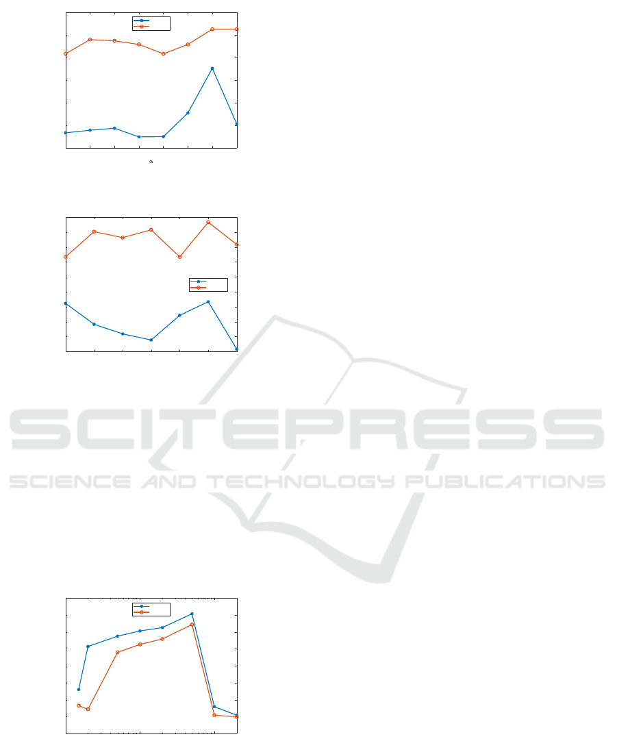
In the first experiment, we evaluate the effect of
the parameter α. Fig. 1 shows the variation of accu-
racy respect to the variation of the parameter α. As
we observe, the accuracy for the test samples is rela-
tively fix and does not vary when α varies, however,
the unlabeled data has a higher variance. Also, the
accuracy has its best values when α is 0.7.
In the second experiment, the effect of w
max
is
evaluated. Fig. 2 shows the effect of varying this pa-
rameter on the accuracy. We can see that the accuracy
1
http://archive.ics.uci.edu/ml/datasets/Covertype
VISAPP 2024 - 19th International Conference on Computer Vision Theory and Applications
706

0.1 0.2 0.3 0.4 0.5 0.6 0.7 0.8
54
56
58
60
62
64
66
Accuracy
Unlabel
Test
Figure 1: Performance of the proposed method versus α pa-
rameter on the MNIST database with five labeled samples.
50 100 150 200 250 300 350
W
max
56
57
58
59
60
61
62
63
64
65
Accuracy
Unlabel
Test
Figure 2: Performance of the proposed method versus w
max
parameter on the MNIST database with five labeled sam-
ples.
has its highest value when w
max
is 300. Moreover, we
observe that the accuracy does not follow the same
trend specially when w
max
is lower than 250.
Thirdly, we evaluate the effect of varying number
of the anchors. In Fig. 3, we have plotted the accuracy
when the number of anchors varies in the range [10
20 50 100 200 500 1000 2000]. As we can see the ac-
curacy increases as the number of anchors increases,
however, we observe that the accuracy suddenly drops
as we use more than 1000 anchors.
10
1
10
2
10
3
Number Of Anchors
0
10
20
30
40
50
60
70
80
Accuracy
Unlabel
Test
Figure 3: Performance of the proposed method versus the
number of anchors on the MNIST database with five labeled
samples.
4.2 Comparison with Other Methods
For comparison, we used two recently proposed meth-
ods, r-FME(Qiu et al., 2019) and SGRFME(Ibrahim
et al., 2023). Since we are in semi-supervised context,
in the training data we have labeled and unlabaled
samples. Hence, for the number of labeled samples
per class, in the Covtype database, we set l to 30, 50,
and 70 and for MNIST we set l to 5 and 20.
In these experiments, we fixed w
min
to one, α to
0.7, and w
max
to 300. For the diagonal U
l
matrix, we
set the first l elements to the weights obtained by To-
toro values (i.e., w
k
) and the rest to zero. For µ, γ,
λ, and ρ, we select one split of labeled and unlabeled
data and scan the parameters to find the best combi-
nations. Then we fix the obtained parameters for the
rest of the experiments.
Table 1 shows the average and standard devia-
tion for 20 random combinations of labeled and unla-
beled samples on Covtype an MNIST databases. We
use bold font for the highest accuracy. As we ob-
serve, the average accuracy of the proposed method is
higher compared to other competing methods includ-
ing SGRFME, which shows the effect of the adaptive
weighting of SGRFME algorithm. Also, the standard
deviation of the proposed method is lower, showing a
more stable accuracy compared to other methods. We
observe this behavior for both databases which shows
that there is no bias toward a specific database for the
outperformance of the proposed method. Also, we
can see that even though the training database is the
same, when we increase the number of labeled sam-
ples, we have an increase in the accuracy for all meth-
ods. However, the proposed method keeps its outper-
formance in different numbers of labeled samples.
4.3 Confusion Matrix
We calculate the confusion matrix of the proposed
method. We select one split of MNIST database with
5 labeled samples and estimate the labels of the un-
labeled set and test set. We then plot the confusion
and report the precision, recall, and F1 score for each
class in Table 2. Moreover, we report the macro preci-
sion, macro recall, and macro F1 score. Macrometrics
(Precision, Recall, and F1 score) are calculated by av-
eraging the metrics across all classes.
5 CONCLUSION
In this article, we tackle the problem of topology im-
balance in graphs. We adopted the Renode technique
to assign weights to the labeled samples. To do so,
Large Scale Graph Construction and Label Propagation
707

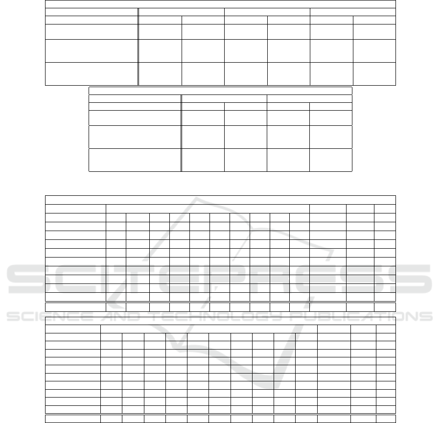
Table 1: Average accuracy with standard deviation for the proposed method and two recent methods (r-FME and SGRFME)
obtained on 20 random combinations of labeled and unlabeled samples.
Covtype
Method 30 labeled samples 50 labeled samples 70 labeled samples
Unlabeled Test Unlabeled Test Unlabeled Test
r-FME (Qiu et al., 2019)
47.70 ± 3.20 45.88 ± 3.87 49.54 ± 1.78 50.01 ± 3.14 51.89 ± 2.08 53.36 ± 2.74
(10
15
,10
0
) (10
9
,10
−3
) (10
24
,10
6
) (10
9
,10
−3
) (10
9
,10
−3
) (10
9
,10
−3
)
SGRFME (Ibrahim et al., 2023)
51.00 ± 2.02 49.62 ± 2.39 52.39 ± 1.82 52.23 ± 1.97 54.62 ± 0.95 54.11 ± 1.24
(10
24
,10
−12
(10
24
,10
−12
(10
12
,10
24
(10
6
,10
3
(10
18
,10
6
(10
6
,10
3
10
18
,10
−12
) 10
−12
,10
18
) 10
24
,10
12
) 10
12
,10
0
) 10
3
,10
24
) 10
12
,10
24
)
W-SGRFME
52.70 ± 2.58 52.91 ± 2.26 53.38 ± 0.84 53.41 ± 1.74 55.16 ± 0.76 54.77 ± 0.66
(10
24
,10
−12
(10
24
,10
−12
(10
12
,10
24
(10
6
,10
3
(10
18
,10
6
(10
6
,10
3
10
−12
,10
18
) 10
−12
,10
18
) 10
24
,10
12
) 10
12
,10
0
) 10
3
,10
24
) 10
12
,10
24
)
MNIST
Method 5 labeled samples 20 labeled samples
Unlabeled Test Unlabeled Test
r-FME (Qiu et al., 2019)
64.47 ± 2.24 57.82 ± 4.31 70.39 ± 1.05 67.61 ± 3.07
(10
21
,10
−12
) (10
0
,10
3
) (10
21
,10
−12
) (10
9
,10
0
)
SGRFME (Ibrahim et al., 2023)
65.29 ± 1.82 58.27 ± 4.42 71.22 ± 0.83 68.08 ± 2.95
(10
9
,10
0
(10
−24
,10
3
(10
9
,10
0
(10
−24
,10
3
10
−24
,10
15
) 10
−12
,10
9
) 10
−24
,10
15
) 10
−12
,10
9
)
W-SGRFME
66.09 ± 1.42 59.17 ± 4.12 71.72 ± 1.01 69.17 ± 2.89
(10
9
,10
0
(10
−24
,10
3
(10
9
,10
0
(10
−24
,10
3
10
−24
,10
15
) 10
−12
,10
9
) 10
−24
,10
15
) 10
−12
,10
9
)
Table 2: Confusion Matrix, Precision, Recall, and F1 of the proposed method on the MNIST database (5 labeled samples).
Unlabeled samples
Predicted Precision Recall F1
Class 1 (Actual) 846 0 6 4 0 1 33 2 14 59 0.85 0.87 0.86
Class 2 (Actual) 0 1050 0 0 2 0 3 28 0 2 0.93 0.96 0.95
Class 3 (Actual) 9 1 547 95 15 146 40 22 74 120 0.55 0.51 0.53
Class 4 (Actual) 3 0 48 307 1 170 3 2 7 12 0.30 0.55 0.38
Class 5 (Actual) 7 43 92 9 900 31 28 306 14 29 0.92 0.61 0.73
Class 6 (Actual) 2 0 71 552 4 498 6 3 8 27 0.55 0.42 0.48
Class 7 (Actual) 84 0 101 18 2 34 779 9 71 114 0.79 0.64 0.70
Class 8 (Actual) 3 29 28 0 25 5 13 661 2 11 0.63 0.85 0.72
Class 9 (Actual) 10 0 24 18 0 3 7 0 645 50 0.66 0.85 0.74
Class 10 (Actual) 23 1 76 19 25 16 74 11 140 568 0.57 0.59 0.58
Macro 0.69 0.68 0.67
Test samples
Predicted Precision Recall F1
Class 1 (Actual) 4679 1 60 21 14 40 805 71 18 581 0.94 0.74 0.83
Class 2 (Actual) 7 4981 37 0 41 19 198 884 33 40 0.88 0.79 0.84
Class 3 (Actual) 2 4 1184 37 35 63 56 54 21 195 0.23 0.71 0.35
Class 4 (Actual) 59 1 1168 4070 56 2827 178 75 80 752 0.79 0.43 0.56
Class 5 (Actual) 37 620 683 49 4213 87 175 1072 81 264 0.86 0.57 0.69
Class 6 (Actual) 15 0 499 696 7 1092 296 10 24 89 0.24 0.40 0.30
Class 7 (Actual) 33 0 67 21 0 39 1920 8 4 31 0.38 0.90 0.54
Class 8 (Actual) 16 11 409 27 454 126 82 3035 10 123 0.58 0.70 0.63
Class 9 (Actual) 87 0 818 148 36 76 1154 10 4598 1484 0.94 0.54 0.69
Class 10 (Actual) 1 0 40 40 12 148 68 2 7 1398 0.28 0.81 0.41
Macro 0.61 0.66 0.58
we used anchors as data representatives and modified
the Renode method to extend the idea of topological
imbalance for large scale databases. Then we adopted
the label estimation error term to insert these weights
into our objective function. Our experimental results
on two large databases show that the proposed method
has a higher average accuracy and lower standard de-
viation compared to two recently proposed methods
namely r-FME and SGRFME. On the other hand, due
to the iterative nature of the proposed method, it has
a higher computational complexity than its competi-
tive methods. Moreover, the relatively large number
of parameters to be tuned is another weakness of the
proposed method. Hence, as a future work, we focus
on the automatic tuning of these parameters. Also, re-
duction of the running time is another track to follow.
REFERENCES
Aromal, A., M. Rasool, A., Dubey, A., and Roy, B. N.
(2021). Optimized weighted samples based semi-
supervised learning. In 2021 Second International
Conference on Electronics and Sustainable Commu-
nication Systems (ICESC), pages 1311–1318.
Belkin, M., Niyogi, P., and Sindhwani, V. (2006). Manifold
regularization: A geometric framework for learning
from labeled and unlabeled examples. The Journal of
Machine Learning Research, 7:2399–2434.
VISAPP 2024 - 19th International Conference on Computer Vision Theory and Applications
708

Bosaghzadeh, A., Moujahid, A., and Dornaika, F. (2013).
Parameterless local discriminant embedding. Neural
Processing Letters, 38.
Bui, Q.-T., Vo, B., Do, H.-A. N., Hung, N. Q. V., and Snasel,
V. (2020). F-mapper: A fuzzy mapper clustering al-
gorithm. Knowledge-Based Systems, 189:105107.
Bui, Q.-T., Vo, B., Snasel, V., Pedrycz, W., Hong, T.-P.,
Nguyen, N.-T., and Chen, M.-Y. (2021). Sfcm: A
fuzzy clustering algorithm of extracting the shape in-
formation of data. IEEE Transactions on Fuzzy Sys-
tems, 29(1):75–89.
Chen, D., Lin, Y., Zhao, G., Ren, X., Li, P., Zhou, J.,
and Sun, X. (2021). Topology-imbalance learning
for semi-supervised node classification. Advances in
Neural Information Processing Systems, 34:29885–
29897.
Chen, X., Yu, G.-X., Tan, Q., and Wang, J. (2019).
Weighted samples based semi-supervised classifica-
tion. Applied Soft Computing, 79:46–58.
Collobert, R., Sinz, F., Weston, J., and Bottou, L. (2006).
Large scale transductive svms. Journal of Machine
Learning Research, 7:1687–1712.
Cui, B., Xie, X., Hao, S., Cui, J., and Lu, Y. (2018).
Semi-supervised classification of hyperspectral im-
ages based on extended label propagation and rolling
guidance filtering. Remote Sensing, 10(4).
Dornaika, F., Baradaaji, A., and El Traboulsi, Y. (2021).
Semi-supervised classification via simultaneous label
and discriminant embedding estimation. Information
Sciences, 546:146–165.
Hamilton, W. L., Ying, R., and Leskovec, J. (2017). Induc-
tive representation learning on large graphs. In Pro-
ceedings of the 31st International Conference on Neu-
ral Information Processing Systems, NIPS’17, page
1025–1035, Red Hook, NY, USA. Curran Associates
Inc.
He, K., Zhang, X., Ren, S., and Sun, J. (2015). Deep
residual learning for image recognition. CoRR,
abs/1512.03385.
Ibrahim, Z., Bosaghzadeh, A., and Dornaika, F. (2023).
Joint graph and reduced flexible manifold embedding
for scalable semi-supervised learning. Artificial Intel-
ligence Review, 56:9471–9495.
Kang, Z., Peng, C., Cheng, Q., Liu, X., Peng, X., Xu, Z.,
and Tian, L. (2021). Structured graph learning for
clustering and semi-supervised classification. Pattern
Recognition, 110:107627.
Long, Y., Li, Y., Wei, S., Zhang, Q., and Yang, C. (2019).
Large-scale semi-supervised training in deep learn-
ing acoustic model for asr. IEEE Access, 7:133615–
133627.
Nie, F., Cai, G., and Li, X. (2017). Multi-view cluster-
ing and semi-supervised classification with adaptive
neighbours. In Thirty-First AAAI Conference on Arti-
ficial Intelligence.
Nie, F., Wang, X., Jordan, M. I., and Huang, H. (2016). The
constrained laplacian rank algorithm for graph-based
clustering. In AAAI Conference on Artificial Intelli-
gence.
Nie, F., Xu, D., Tsang, I. W., and Zhang, C. (2010). Flex-
ible manifold embedding: A framework for semi-
supervised and unsupervised dimension reduction.
IEEE Transactions on Image Processing, 19(7):1921–
1932.
Qiu, S., Nie, F., Xu, X., Qing, C., and Xu, D. (2019). Ac-
celerating flexible manifold embedding for scalable
semi-supervised learning. IEEE Transactions on Cir-
cuits and Systems for Video Technology, 29(9):2786–
2795.
Sindhwani, V. and Niyogi, P. (2005). Linear manifold regu-
larization for large scale semi-supervised learning. In
Proc. of the 22nd ICML Workshop on Learning with
Partially Classified Training Data.
Sindhwani, V., Niyogi, P., Belkin, M., and Keerthi, S.
(2005). Linear manifold regularization for large scale
semi-supervised learning. Proc. of the 22nd ICML
Workshop on Learning with Partially Classified Train-
ing Data.
Song, Z., Yang, X., Xu, Z., and King, I. (2022). Graph-
based semi-supervised learning: A comprehensive re-
view. IEEE Transactions on Neural Networks and
Learning Systems, pages 1–21.
Tu, E., Wang, Z., Yang, J., and Kasabov, N. (2022).
Deep semi-supervised learning via dynamic anchor
graph embedding in latent space. Neural Networks,
146:350–360.
Wang, J., Yang, J., Yu, K., Lv, F., Huang, T., and Gong,
Y. (2010). Locality-constrained linear coding for im-
age classification. In IEEE Conference on Computer
Vision and Pattern Recognition.
Wang, M., Fu, W., Hao, S., Tao, D., and Wu, X. (2016).
Scalable semi-supervised learning by efficient anchor
graph regularization. IEEE Transactions on Knowl-
edge and Data Engineering, 28(7):1864–1877.
Wang, Z., Wang, L., Chan, R. H., and Zeng, T. (2019).
Large-scale semi-supervised learning via graph struc-
ture learning over high-dense points.
Wang, Z., Zhang, L., Wang, R., Nie, F., and Li, X. (2022).
Semi-supervised learning via bipartite graph construc-
tion with adaptive neighbors. IEEE Transactions on
Knowledge and Data Engineering, pages 1–1.
Wu, X., Zhao, L., and Akoglu, L. (2019). A quest for struc-
ture: Jointly learning the graph structure and semi-
supervised classification.
Yuan, Y., Li, X., Wang, Q., and Nie, F. (2021). A semi-
supervised learning algorithm via adaptive laplacian
graph. Neurocomputing, 426:162–173.
Zhu, X. and Lafferty, J. (2005). Harmonic mixtures: com-
bining mixture models and graph-based methods for
inductive and scalable semi-supervised learning. In
Machine Learning, Proceedings of the Twenty-Second
International Conference (ICML 2005), Bonn, Ger-
many, August 7-11, 2005.
Large Scale Graph Construction and Label Propagation
709