A Supervised Machine Learning Approach for the Vehicle Routing

Problem

Sebastian Ammon

, Frank Phillipson

1,2 a

and Rui Jorge Almeida

1 b

School of Business and Economic, Maastricht University, Maastricht, The Netherlands

TNO, The Hague, The Netherlands

Keywords:

Supervised Machine Learning, Vehicle Routing Problem, Graph Convolutional Network, Optimisation.

Abstract:

This paper expands on previous machine learning techniques applied to combinatorial optimisation problems,

to approximately solve the capacitated vehicle routing problem (VRP). We leverage the versatility of graph

neural networks (GNNs) and extend the application of graph convolutional neural networks, previously used

for the Travelling Salesman Problem, to address the VRP. Our model employs a supervised learning tech-

nique, utilising solved instances from the OR-Tools solver for training. It learns to provide probabilistic

representations of the VRP, generating ﬁnal VRP tours via non-autoregressive decoding with beam search.

This work shows that despite that reinforcement learning based autoregressive approaches have better perfor-

mance, GNNs show great promise to solve complex optimisation problems, providing a valuable foundation

for further reﬁnement and study.

1 INTRODUCTION

The vehicle routing problem (VRP) is a classical and

complex combinatorial optimisation problem in the

ﬁeld of operations research (OR). At its core, the

problem involves ﬁnding the most efﬁcient routes for

a ﬂeet of vehicles to visit a set of locations, while sat-

isfying operational constraints. It is the generalised

variant of the travelling salesman problem (TSP), for

which there is only one vehicle (travelling salesman).

The VRPs complexity and relevance across various

sectors such as transportation, logistics, and supply

chain management make it a signiﬁcant subject. For

example, the problem has practical applications in

last-mile package delivery, the operations carried out

by companies such as DPD, UPS and FedEx among

others. With demand for last-mile delivery expected

to grow by 78% by 2030, the world’s top 100 cities

(Hillyer, 2020) are expected to see an increase in de-

livery vehicles and therefore carbon emissions. Thus,

improvements in route optimisation can have a posi-

tive impact on the global carbon footprint. This makes

it important to study different views and approaches

to realise these improvement in the near future.

To solve VRPs optimally, an approach like linear

https://orcid.org/0000-0003-4580-7521

https://orcid.org/0000-0002-5844-0768

programming can be used to solve small-sized prob-

lem instances. However obtaining optimal solutions

is challenging when the problem size increases due to

the NP-hard nature (Archetti et al., 2011). To miti-

gate this issue, heuristic methods such as the Clarke

& Wright’s savings algorithm (Clarke and Wright,

1964) trade solution quality for reduced computa-

tion time, see (Konstantakopoulos et al., 2020) for a

survey of these methods. Developing such heuristic

methods is not trivial and often require experts do-

main knowledge, problem-speciﬁc assumptions and

constraints. Furthermore, these heuristics fail to gen-

eralise to small changes in the inputs and need to be

solved from scratch (Bogyrbayeva et al., 2022).

In recent years, machine learning (ML), with its

ability to learn from and make decisions based on

data, has emerged as a promising tool for solving

complex problems. The strength of using ML is its

ability to “learn” approximations of functions, with-

out the need to explicitly formulate these functions

(Bogyrbayeva et al., 2022). While combinatorial op-

timisation problems have traditionally been part of the

OR community, this incredible versatility of ML has

led to an increased interest in the ML community to

tackle combinatorial optimisation problems without

explicitly exploiting the structures of the mathemat-

ical models (Bai et al., 2023).

This paper aims to advance the ML and OR

364

Ammon, S., Phillipson, F. and Almeida, R.

A Supervised Machine Learning Approach for the Vehicle Routing Problem.

DOI: 10.5220/0012430000003639

Paper published under CC license (CC BY-NC-ND 4.0)

In Proceedings of the 13th International Conference on Operations Research and Enterprise Systems (ICORES 2024), pages 364-371

ISBN: 978-989-758-681-1; ISSN: 2184-4372

communities’ intersection by using graph neural net-

works (GNNs) to address the challenging capacitated

VRP. In the literature, two main methods are preva-

lent: supervised and reinforcement learning. Super-

vised learning (SL) approximates VRP solutions us-

ing training data, while reinforcement learning is em-

ployed when such solutions are unavailable. We in-

vestigate the effectiveness of a supervised ML ap-

proach in solving the capacitated VRP, which is an

underexplored area, as discussed in the following sec-

tion. To accomplish this, we extend the work of (Joshi

et al., 2019), who applied a graph convolutional neu-

ral network (GCNN) to the TSP.

2 RELATED WORK

In 1985, Hopﬁeld and Tank were the ﬁrst to demon-

strate the use of a neural network to solve the TSP

(Hopﬁeld and Tank, 1985), which is related to VRP.

They used the Hopﬁeld neural network converting

the objective function of the problem into the en-

ergy function of the neural network. This allowed the

network to ﬁnd locally optimal solutions to the TSP

with up to 30 nodes (cities). Most of the early litera-

ture in this area focused on tackling the TSP through

Hopﬁeld networks and self-organising feature maps

(Smith, 1999).

Over the last two decades, there has been increas-

ing interest in using neural networks to solve com-

binatorial optimisation problems, including a wide

range of routing problems and their variants. A no-

table contribution is the introduction of the pointer

network by (Vinyals et al., 2015), which consists of an

encoder and decoder implemented as recurrent neu-

ral networks (RNNs). Using SL, the model is able

to generate a probability distribution (heat-map) over

the cities to be visited. During the inference stage,

beams search is used to generate valid tours for the

TSP. Although this approach gave promising results

for the TSP instance with up to 30 nodes, it faced

challenges when handling larger instances of up to

40 or 50 nodes. To address this limitation, (Bello

et al., 2017) extended the approach by incorporating

reinforcement learning with an actor-critic scheme,

which led to improved performance for TSP instances

with up to 100 nodes. This work was further ex-

tended by (Deudon et al., 2018) and (Kool et al.,

2019). Their models performs comparable to meth-

ods such as Concorde, LKH3 and Gurobi, and out-

performs approaches by (Vinyals et al., 2015), (Bello

et al., 2017), (Khalil et al., 2017) and (Nowak et al.,

2017) for the TSP. To address the dynamic nature of

the VRP, (Peng et al., 2020) extend (Kool et al., 2019)

with a dynamic attention model consisting of a dy-

namic encoder-decoder architecture. Another notable

contribution for solving VRPs with neural networks is

the work done by (Nazari et al., 2018). This allowed

them to solve the capacitated VRP and its variants;

split-delivery and stochastic VRPs. The model was

trained with an actor-critic scheme, and the solution

was obtained by beam search.

Several approaches exist that employ SL instead

of reinforcement learning. For instance, (Prates et al.,

2019) trains a GNN to determine if a TSP tour with a

cost below a given threshold exists. (Nowak et al.,

2017) and (Joshi et al., 2019) take an end-to-end

approach, training GNN and GCNN models to out-

put probable edge connections between nodes non-

autoregressively, converting these connections into

valid TSP tours using beam search. While Joshi’s ap-

proach outperforms autoregressive methods (Vinyals

et al., 2015; Bello et al., 2017; Khalil et al., 2017;

Kool et al., 2019), it faces limitations as instance

sizes increase. The work in (Fu et al., 2021) ad-

dresses large-scale TSPs by dividing the graph into

subgraphs, training a model to produce probability

matrices for each subgraph, and using Monte Carlo

tree search (MCTS) to ﬁnd solutions. Duan (Duan

et al., 2020) combines reinforcement and SL, using a

GCNN encoder and two decoders to effectively solve

VRPs based on real-world data.

There are hybrid methods that combine ML with

non-learning techniques. (Kool et al., 2022) replaces

beam search with dynamic programming to solve TSP

and VRP, tackles (Li et al., 2021) large-scale VRP by

iteratively improving solutions with SL and a mixed

integer linear solver and (Hottung and Tierney, 2020)

uses a deep neural network trained by policy gradient

reinforcement learning to enhance large neighbour-

hood search (LNS) operators, outperforming other

LNS algorithms and previous ML-based methods.

In this work, we propose to extend the work by

(Joshi et al., 2019) to address the capacitated VRP.

3 METHODOLOGY

3.1 General Overview

Given a VRP graph with n nodes as input, our ap-

proach is to train a GNN through SL to output an

adjacency matrix P = {p

i j

}

i, j=0

corresponding to the

tours of the VRP. Each entry p

i j

∈ [0, 1] represents

the probability that nodes i and j are connected in

the VRP solution. We use beam search to decode the

probabilistic matrix P and output the ﬁnal sequence

of nodes of the VRP tours.

A Supervised Machine Learning Approach for the Vehicle Routing Problem

365

Our proposed model

uses the GCNN presented

by (Joshi et al., 2019) for the TSP, but we adapt

the network architecture to support the VRP. The

model takes node and edge features as input and

learns an initial representation (embedding) vector for

each node and edge. The embedding vectors are

updated by passing through a series of graph con-

volution layers and exchanging information between

adjacent nodes and edges. This is known as the

message-passing framework, where at each layer (it-

eration) nodes and edges aggregate information (the

messages) from their local neighbourhood (Hamilton,

2020). This is the main idea that distinguishes stan-

dard neural networks from GNNs. This is a power-

ful mechanism because after passing through L layers,

node i and edge (i j) will have aggregated feature in-

formation from their L-hop neighbours into their own

feature vectors. This allows the GNN to incorporate

the structural (graph-like) nature of the problem.

The edge embedding vector from the last graph

convolution layer is passed through a multilayer per-

ceptron (MLP) to independently predict for each edge

whether it is part of the VRP solution or not. Finally,

we use a decoding strategy known as beam search to

take the edge predictions and generate a ﬁnal VRP so-

lution.

3.2 Graph Convolutional Network for

Vehicle Routing Problem

3.2.1 Input Layer

The model receives node and edge features as input.

The input layer is responsible for projecting the ini-

tial feature vectors into a h-dimensional latent space.

We extend the approach of (Joshi et al., 2019) to sup-

port VRP by adding two additional node features and

removing one of the edge features, the edge type indi-

cator matrix. Each node i has an input feature vector

= [x

], where x

is the two-dimensional loca-

tion, q

is the demand, and t

is a node token. For the

depot node t

= 1 and for all other nodes t

= 0. With-

out loss of generality, we normalise the demand with

respect to the vehicle capacity per dataset. The node

feature vector is embedded in h dimensional space:

= A

+ b

(1)

where A

∈ R

h×4

and and b

are a trainable parameter

matrix and bias term, respectively. The Euclidean dis-

tance d

i j

is embedded as a h-dimensional edge feature

vector β

i j

deﬁned as

i j

= A

i j

+ b

(2)

Code and data are available at https://github.com/seb

ammon/vrp-thesis

Figure 1: Illustration of how feature vectors at the next layer

ℓ + 1 aggregate information from their neighbours at the

previous layer ℓ. The dashed red and blue lines show the in-

formation ﬂow for the node and edge features, respectively.

Adapted from (Joshi et al., 2019).

where A

∈ R

h×1

and b

are a trainable parameter ma-

trix and bias term, respectively. (Joshi et al., 2019)

also deﬁne an edge type indicator matrix to signal k-

nearest neighbours, self-connections and normal edge

connection types. They argue that this speeds up

learning since connected nodes in the TSP solution

are often in close proximity. We experimented with

this matrix but did not ﬁnd that its presence improved

the learning process or the quality of the solution.

3.2.2 Graph Convolution Layer

The graph convolution layer is responsible for updat-

ing the node and edge feature vectors by aggregating

information from their local neighbourhoods. Let x

ℓ

and e

ℓ

i j

denote the node and edge feature vectors at

layer ℓ, for ℓ = 0, . . . , L, associated with node i and

edge (i j) respectively. In the input layer, x

ℓ=0

= α

and e

ℓ=0

i j

= β

i j

. The information aggregation for x

ℓ

and e

ℓ

i j

, at the next layer ℓ + 1 is:

ℓ+1

= UPD

ℓ



ℓ

, AGG

ℓ



{(x

ℓ

, η

ℓ

i j

),∀ j ∈ N (i)}



ℓ+1

i j

= UPD

ℓ



ℓ

i j

, AGG

ℓ



ℓ

, x

ℓ



where UPDATE (UPD) and AGGREGATE (AGG)

are arbitrary differentiable functions (Hamilton,

2020), N (i) is the set of neighbours for node i (which

are all nodes, since we use a fully connected input

graph), and η

ℓ

i j

are learnable edge gates. The edge

gates allow the model to learn the relative importance

of each neighbour of node i when aggregating their

information. Figure 1 shows the ﬂow of information

between nodes and edges from one layer to the next.

More concretely, (Joshi et al., 2019) deﬁne the

node and edge feature vectors as:

ICORES 2024 - 13th International Conference on Operations Research and Enterprise Systems

366

ℓ+1

= x

ℓ

+ ReLU









ℓ

∑

j∈N (i)

ℓ

i j

⊙W

ℓ









ℓ

i j

σ(e

ℓ

i j

)

∑

′

∈N (i)

σ(e

ℓ

i j

′

) + ε

ℓ+1

i j

= e

ℓ

i j

+ ReLU



ℓ

i j

ℓ



where W

ℓ

∈ R

h×h

are trainable pa-

rameter matrices, σ is the sigmoid activation func-

tion, ⊙ is the Hadamard element-wise product, ε is

a small value, ReLU is the rectiﬁed linear unit func-

tion and BN applies the batch normalisation (Ioffe and

Szegedy, 2015). Due to the symmetric nature of the

VRP, W

ℓ

= W

ℓ

3.2.3 Multilayer Perceptron Classiﬁer

An MLP is a fully connected feedforward artiﬁcial

neural network consisting of an input layer, hidden

layers and an output layer. The MLP is used to inde-

pendently compute the edge probability p

i j

, i.e., the

probability that edge (i j) is active in the ﬁnal VRP

solution, from the ﬁnal edge feature vector e

ℓ

i j

= MLP(e

ℓ

i j

) (3)

The h dimensional hidden layers of the MLP are con-

nected via the ReLU activation function. We apply a

softmax activation function to the last layer to trans-

late it to the range [0,1].

3.2.4 Loss Function

The model is trained in a supervised fashion by min-

imising the weighted cross-entropy loss between the

edges P = {p

i j

}

i, j=0

predicted by the model and the

ground truth edges T = {t

i j

}

i, j=0

from the solver,

where n is the number of nodes. Cross-entropy is a

loss function commonly used for binary classiﬁcation

tasks, which is essentially what this problem is – an

edge can be either active or inactive – deﬁned as:

Loss

i j

∑

c=0

log(p

i j

i j,c

, (4)

where I

i j,c

is deﬁned as the indicator function that

takes the value of 1 if class is c, and 0 otherwise.

Since the adjacency matrix of VRP is usually

sparse, i.e., there are many more inactive edges than

active ones, (Joshi et al., 2019) provide the cross-

entropy with the weights for each class. They state

that the classiﬁcation becomes highly unbalanced to-

wards the negative class as the problem size increases

and appropriate class weights are needed to mitigate

this issue. The class weights for each class c, active

or inactive, are calculated per dataset by:

∑

c=0

2 · I

where I

∑

i, j=0

i j,c

is the number of occurrences

of class c,

∑

c=0

is the number of instances in the

dataset. The loss per training epoch is calculated as

the average loss over all mini-batches.

3.3 Beam Search Decoding

The model outputs a probabilistic adjacency matrix of

edges, where each entry p

i j

indicates the probability

that the edge (i j) is part of the VRP solution. This

matrix cannot be converted directly into VRP routes,

e.g., using the argmax function, as this may result in

invalid tours with missing or redundant edges. A de-

coder is required to deal with this.

Beam search is a limited-width breadth-ﬁrst

search algorithm commonly used to generate highly

probable output sequences for natural language pro-

cessing tasks (Medress et al., 1977). It iteratively ex-

pands the next most likely nodes, keeping only the b

most likely sequences found so far, where b refers to

the beam width. This is a greedy algorithm as it only

keeps a limited number of possible solutions.

Beam search decoding can be used to generate

tours (a sequence of nodes) by expanding the most

probable edges between nodes to form a tour. Accord-

ing to (Joshi et al., 2019), the probability of a partial

tour π

′

is based on the chain rule of probability as:

p(π

′

) =

∏

′

∼i

′

∈π

′

(5)

where each node j

′

follows node i

′

in the partial tour

′

. Starting from the ﬁrst node i, the beam search ex-

pands the b most probable edges from the probability

adjacency matrix by exploring the neighbours of the

node. At each iteration, the next b most probable par-

tial tours are expanded until all nodes have been vis-

ited. To ensure that nodes are not visited more than

once, (Joshi et al., 2019) use a masking strategy to

hide previously visited nodes.

While the approach of (Joshi et al., 2019) works

well for a single TSP tour, it is not directly applica-

ble to VRP because it does not consider two points.

First, the fact that each vehicle requires a tour; second,

the capacity constraint of the vehicles. To address

the ﬁrst point, we adapt the masking strategy to hide

the depot node only when it has been visited K many

times, where K is the number of vehicles. The other

nodes are masked as soon as they have been visited.

A Supervised Machine Learning Approach for the Vehicle Routing Problem

367

This translates into a tour per vehicle as follows: as-

suming a partial tour π

′

= {0, 3, 2, 4, 0, 1, 6, 5}, where

K = 2 and all n = 6 nodes have been visited, then

the tours for the two vehicles can be extracted as

= {0,3,2,4,0} and R

= {0,1,6,5,0}.

To take into account the second point, namely the

capacity constraints of the vehicles, we keep track of

the remaining capacity of the vehicle after visiting the

nodes of the partial tour. When expanding the next b-

most probable partial tours, we hide nodes where the

demand exceeds the remaining capacity of the vehicle

(current tour), which is reset when the depot node is

visited. We follow two beam search approaches to

construct the ﬁnal tours.

3.3.1 Standard Beam Search

Following the description above, we generate b most

probable tours by specifying the beam width param-

eter. From these tours we select the one with the

highest probability in Equation 5. However, the most

probable tour is not guaranteed to be the shortest. For

this reason, we only use this approach during the vali-

dation phase when training the model. Intuitively, the

model improves its predictions as the probability of

promising edges should increase while the probabil-

ity of less promising edges should decrease. Using

the most promising tour during training gives an indi-

cation for model improvement.

3.3.2 Shortest Tour Heuristic

In this approach, instead of selecting the most proba-

ble tour among the candidates, we select the shortest

tour by evaluating and comparing the distance of each

tour. This algorithm takes considerably more time to

execute, so we only use it after training as a ﬁnal eval-

uation of the model’s performance.

4 EXPERIMENTAL DESIGN

4.1 Data Setup

The data is based on the VRP in the two-dimensional

Euclidean plane. Given an input graph, we deﬁne a

VRP instance with n customers (nodes) as a sequence

of tuples S = {(x

)}

i=0

, where x

∈ [0, 1]

is the lo-

cation in the unit square and q

∈ {1, ..., 9} is the de-

mand. We add a special node at index 0, called the

depot, with location x

and demand q

= 0. Addition-

ally we deﬁne the cost of each edge between nodes i

and j, to be the Euclidean distance d

i j

= ∥x

− x

∥

The goal is to ﬁnd a set of routes (vehicles) that

start and stop at the depot, visiting each customer only

once (across all routes), while minimising the total

distance travelled. All vehicles are homogeneous and

each vehicle has a (positive) capacity (κ) that may not

be exceeded, so

∑

i∈R

≤ κ, where R

is the set of

nodes visited by vehicle k ∈ {1,...,K}.

To solve an instance to create training and valida-

tion instances, we use the VRP solver from the open

source software suite OR-Tools (Perron and Furnon,

2023). The solutions it ﬁnds are not guaranteed to

be optimal, as the solver uses heuristics along with

metaheuristics to ﬁnd approximate solutions. As in-

put to the solver we give it a n × n distance matrix

D = {d

i j

}

i, j=0

, the customer demand q

, the depot

node index i = 0, the vehicle capacity κ and the to-

tal number of available vehicles K. Additionally, we

need to specify the heuristic and metaheuristic to be

used by the solver. Here we used the path cheapest

arc heuristic, as it is a constructive heuristic that incre-

mentally builds the routes from the depot by adding

the next node that produces the cheapest route seg-

ment (Perron and Furnon, 2023). For the metaheuris-

tic, we opt for Guided Local Search (Voudouris et al.,

2010), which guides the solver to escape local min-

ima. The stopping criterion used for this approach is

a time limit (in seconds). In order for the solver to

consistently ﬁnd good solutions for different problem

sizes (number of nodes), we adjust the time limit for

each generated dataset.

The obtained set of routes {R

}

k=1

are then con-

verted into an adjacency matrix T

= {t

i j

}

i, j=0

, which

constitutes target matrix for model training. For each

entry in the target matrix, t

i j

= 1 if nodes i and j are

connected in route R

, and 0 otherwise. Due to the

symmetric nature of VRP, if nodes i and j are con-

nected, then the reverse is also true, hence t

i j

= t

4.2 Training Procedure

To train the ML model, we generate training and vali-

dation data. To explore the ability of the model to gen-

eralise to different problem sizes, we generate three

different datasets, VRP10, VRP20 and VRP50 with

10, 20 and 50 customer nodes respectively. Following

the approach of (Nazari et al., 2018), for each dataset

we set the vehicle capacity to 20, 30 and 40 respec-

tively and the number of available vehicles to 4, 5 and

10. For the datasets VRP10 and VRP20, we generate

and solve 20,000 instances, of which 1,000 instances

are kept as a validation set. We set the time limit for

the metaheuristic to 1 and 3 seconds for each dataset.

For the VRP50 dataset, with the larger 50 node in-

stances, we increase the solver time limit to 8 seconds

in order to obtain better solutions. This marginal in-

crease has a signiﬁcant impact on the running time

ICORES 2024 - 13th International Conference on Operations Research and Enterprise Systems

368

for data generation. Thus, we only generate 10,000

instances, of which 500 are kept for validation. The

model is trained separately on each dataset.

Different models are trained, each dedicated to

one of the following datasets: VRP10, VRP20 and

VRP50. The same hyperparameters are adopted for

all models, allowing a comparative analysis. We use

32 hidden units, 12 GCN layers, 3 MLP layers. The

model is trained by minimising the weighted cross-

entropy loss between the predicted edges and the

ground truth edges for each mini-batch. The loss

minimisation task is performed using the stochas-

tic gradient descent technique and Adam optimiser

(Kingma and Ba, 2015), with a learning rate of 0.001,

50 epochs and a batch size of 64. Each training

and validation dataset is divided into mini-batches of

64 instances. For each epoch of the training phase,

the model makes one pass through the entire training

dataset. Models are trained for 50 epochs. All compu-

tations are performed on the Nvidia T4 GPU provided

by the Google Colab platform.

4.3 Evaluation Procedure

At the end of each epoch of the training process, we

evaluate the performance of the model on the entire

validation set. The predicted edge adjacency matrix

is converted into a valid VRP tour using the standard

beam search strategy described in Section 3.3.1, with

a beam width of b = 10. The most likely of the candi-

date tours is selected. This approach encourages fast

evaluation while still allowing exploration among the

candidate tours to ﬁnd the most likely tour.

To compare the quality of the tours found by the

model with those obtained by the OR-Tools solver, we

use the average optimality gap. Given the length l of

the predicted tour and the length

l of the solver tour,

average optimality gap over m instances is:

∑

i=1



− 1



(6)

For the ﬁnal evaluation of the model, we use the

shortest tour heuristic (see Section 3.3.2) to convert

the edge adjacency matrix into valid VRP tour can-

didates, from which we select the shortest. This al-

lows us to sample routes from the b most likely can-

didates and select the best (shortest) ones. The size of

the beam width b creates a trade-off between execu-

tion time and solution quality. A larger beam width

explores more candidates at the expense of execu-

tion time, while a smaller beam width does the oppo-

site. Figure 2 shows the trade-off between beam width

and solution quality. For the beam width we choose

b = 1280, similar to the choice made by (Joshi et al.,

2019).

Figure 2: Trade-off between the beam width and the qual-

ity of the solution (average optimality gap) for different

datasets.

Table 1: Average optimality gap with respect to OR-Tools

for our model (GCN), the random baseline and the models

of Kool (Kool et al., 2019) and Duan (Duan et al., 2020).

Model

Validation set

VRP10 VRP20 VRP50

OR-Tools 0.00% 0.00% 0.00%

Beam search:

GCN 6.08% 16.06% 20.97%

Duan - -0.41% -2.42%

Kool (greedy) - -0.47% -2.90%

Random baseline 50.99% 105.38% 176.88%

Shortest tour:

GCN 3.28% 8.69% 16.12%

Duan - -0.46% -2.42%

Kool - -2.80% -6.10%

5 RESULTS

5.1 Average Optimality Gap Analysis

Table 1 shows the average optimality gap between the

model (GCN) and the OR-Tools solver evaluated on

all instances of the validation set. For comparison, we

include the average optimality gap obtained using the

standard beam search and shortest tour heuristic de-

coding strategies. We also include the random base-

line results, where we apply the standard beam search

to randomly generated edge probabilities. This com-

parison indicates of whether the model learns mean-

ingful representations for solving VRP instances.

Next, we include results reported by (Kool et al.,

2019) for the attention model and (Duan et al., 2020)

for the GCN node model. They test their models on

VRP20 and VRP50 datasets with instances generated

in a similar way. They do not report their optimality

gap with respect to OR tools.Also, their model does

not have a decoding approach similar to our standard

beam search strategy, so we present their greedy strat-

A Supervised Machine Learning Approach for the Vehicle Routing Problem

369

egy, which is similar to setting b = 1. Our model

clearly outperforms the random baseline by a factor

of about 10, indicating that the model has learned rep-

resentations that are useful for the decoding process.

Across all datasets, the shortest tour heuristic model

outperforms the standard beam search approach. This

is to be expected when sampling more solutions and

selecting the best among them. Second, our model

falls short when compared to the reinforcement learn-

ing approaches of (Kool et al., 2019) and (Duan et al.,

2020). These reinforcement learning models have the

advantage of generating VRP tours in an autoregres-

sive manner, making informed predictions about edge

connections at each decoding step. In contrast, the

non-autoregressive approach of the model generates

edge predictions one-shot, which may not account for

the capacity of the current partial tour.

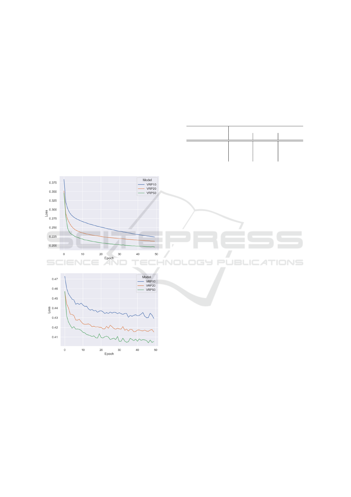
(a) Training loss.

(b) Validation loss.

Figure 3: Training and validation loss for each model over

50 epochs.

5.2 Training Progress and Loss Curves

Figure 3 shows the training progress of the mod-

els over 50 epochs. The training and validation

loss curves follow a similar trajectory, with a sharp

decrease initially and a steady decrease afterwards.

While the training loss follows a smoother path, the

validation loss becomes more irregular, but there’s no

evidence of overﬁtting. The relationship between val-

idation loss and average optimality gap is not straight-

forward, which is challenging for model evaluation

and interpretation.

Table 2: Average optimality gap per model trained and eval-

uated on different problem sizes.

Model

Validation set

VRP10 VRP20 VRP50

GCN (VRP10) 3.28% 18.97% 52.86%

GCN (VRP20) 6.57% 8.69% 28.70%

GCN (VRP50) 5.79% 16.00% 16.12%

5.3 Generalization of the Model

Table 2 explores the generalisation of the model to

different input sizes. Models trained on their respec-

tive datasets tend to outperform models generalizing

to different datasets. Models trained on more com-

plex problems seem to learn representations that are

beneﬁcial when solving less complex problems. The

results suggest that models trained on less complex

problems may not scale well.

6 CONCLUSIONS

In this paper, we introduced a supervised ML ap-

proach for solving VRP, harnessing the power of

GCN. Our model effectively tackles VRP instances

with 10, 20, and 50 customer nodes, delivering

results that signiﬁcantly surpass random baselines.

This success underscores our model’s capacity to ac-

quire the essential knowledge needed for problem-

solving. Nonetheless, reinforcement learning-based

autoregressive methods still outperform our approach.

Our model faces limitations when it comes to lever-

aging prior information for making informed predic-

tions, especially regarding the edges. This becomes

particularly critical in the context of VRP, where con-

sidering vehicle capacity is essential for valid routes.

While SL methods hold promising results, practi-

cal challenges arise. Large amounts of training data

are required, especially for larger and more complex

VRP problem instances. Generating such data de-

mands signiﬁcant time and resources, which increases

with problem complexity increases. Finally, we indi-

rectly demonstrated the expressive power of GNNs by

extending the model architecture for TSP to support

VRP. This shows that there is much potential for us-

ICORES 2024 - 13th International Conference on Operations Research and Enterprise Systems

370

ing GNNs to solve combinatorial optimisation prob-

lems. In order to improve model performance, future

work can focus on different decoding strategies which

are more appropriate the VRP problem complexity by

using an autoregressive decoder.

REFERENCES

Archetti, C., Feillet, D., Gendreau, M., and Speranza, M. G.

(2011). Complexity of the VRP and SDVRP. Trans-

portation Research Part C: Emerging Technologies,

19(5):741–750.

Bai, R. et al. (2023). Analytics and machine learning in ve-

hicle routing research. International Journal of Pro-

duction Research, 61(1):4–30.

Bello, I., Pham, H., Le, Q. V., Norouzi, M., and Bengio,

S. (2017). Neural Combinatorial Optimization with

Reinforcement Learning. arXiv:1611.09940.

Bogyrbayeva, A., Meraliyev, M., Mustakhov, T., and

Dauletbayev, B. (2022). Learning to Solve Vehicle

Routing Problems: A Survey. arXiv:2205.02453.

Clarke, G. and Wright, J. W. (1964). Scheduling of Vehicles

from a Central Depot to a Number of Delivery Points.

Operations Research, 12(4):568–581.

Deudon, M. et al. (2018). Learning Heuristics for the TSP

by Policy Gradient. In Integration of Constraint Pro-

gramming, Artiﬁcial Intelligence, and Operations Re-

search, volume 10848, pages 170–181. Springer In-

ternational Publishing, Cham.

Duan, L. et al. (2020). Efﬁciently Solving the Practical Ve-

hicle Routing Problem: A Novel Joint Learning Ap-

proach. In Proceedings of the 26th ACM SIGKDD

International Conference on Knowledge Discovery &

Data Mining, pages 3054–3063, Virtual Event CA

USA. ACM.

Fu, Z.-H., Qiu, K.-B., and Zha, H. (2021). Generalize a

Small Pre-trained Model to Arbitrarily Large TSP In-

stances. Proceedings of the AAAI Conference on Arti-

ﬁcial Intelligence, 35(8):7474–7482.

Hamilton, W. L. (2020). Graph representation learning.

Morgan & Claypool Publishers.

Hillyer, M. (2020). Urban Deliveries Expected to Add

11 Minutes to Daily Commute and Increase Carbon

Emissions by 30% until 2030 without Effective Inter-

vention by Press releases World Economic Forum.

Hopﬁeld, J. J. and Tank, D. W. (1985). “Neural” computa-

tion of decisions in optimization problems. Biological

Cybernetics, 52(3):141–152.

Hottung, A. and Tierney, K. (2020). Neural Large Neigh-

borhood Search for the Capacitated Vehicle Routing

Problem. Frontiers in Artiﬁcial Intelligence and Ap-

plications, 325 ECAI 2020:443–450.

Ioffe, S. and Szegedy, C. (2015). Batch normalization: Ac-

celerating deep network training by reducing internal

covariate shift. In International conference on ma-

chine learning, pages 448–456. pmlr.

Joshi, C. K., Laurent, T., and Bresson, X. (2019). An Ef-

ﬁcient Graph Convolutional Network Technique for

the Travelling Salesman Problem. In INFORMS An-

nual Meeting 2019, Session on Boosting Combinato-

rial Optimization using Machine Learning.

Khalil, E., Dai, H., Zhang, Y., Dilkina, B., and Song, L.

(2017). Learning combinatorial optimization algo-

rithms over graphs. Advances in neural information

processing systems, 30.

Kingma, D. P. and Ba, J. (2015). Adam: A method for

stochastic optimization. In International Conference

on Learning Representations.

Konstantakopoulos, G. D., Gayialis, S. P., and Kechagias,

E. P. (2020). Vehicle routing problem and related al-

gorithms for logistics distribution: A literature review

and classiﬁcation. Operational research, pages 1–30.

Kool, W. et al. (2022). Deep Policy Dynamic Program-

ming for Vehicle Routing Problems. In Integration of

Constraint Programming, Artiﬁcial Intelligence, and

Operations Research, volume 13292, pages 190–213.

Springer International Publishing, Cham.

Kool, W., van Hoof, H., and Welling, M. (2019). Attention,

Learn to Solve Routing Problems! In International

Conference on Learning Representations (ICLR).

Li, S., Yan, Z., and Wu, C. (2021). Learning to delegate

for large-scale vehicle routing. Advances in Neural

Information Processing Systems, 34:26198–26211.

Medress, M. F. et al. (1977). Speech understanding systems:

Report of a steering committee. Artiﬁcial Intelligence,

9(3):307–316.

Nazari, M. et al. (2018). Reinforcement learning for solv-

ing the vehicle routing problem. Advances in neural

information processing systems, 31.

Nowak, A., Villar, S., Bandeira, A. S., and Bruna, J. (2017).

A Note on Learning Algorithms for Quadratic Assign-

ment with Graph Neural Networks. Proceedings of the

34th International Conference on Machine Learning.

Peng, B., Wang, J., and Zhang, Z. (2020). A deep rein-

forcement learning algorithm using dynamic attention

model for vehicle routing problems. In Artiﬁcial In-

telligence Algorithms and Applications: 11th Interna-

tional Symposium, ISICA 2019, Guangzhou, China,

pages 636–650. Springer.

Perron, L. and Furnon, V. (2023). OR-Tools.

Prates, M. et al. (2019). Learning to Solve NP-Complete

Problems: A Graph Neural Network for Decision

TSP. Proceedings of the AAAI Conference on Arti-

ﬁcial Intelligence, 33(01):4731–4738.

Smith, K. A. (1999). Neural Networks for Combinato-

rial Optimization: A Review of More Than a Decade

of Research. INFORMS Journal on Computing,

11(1):15–34.

Vinyals, O., Fortunato, M., and Jaitly, N. (2015). Pointer

networks. Advances in neural information processing

systems, 28.

Voudouris, C., Tsang, E. P., and Alsheddy, A. (2010).

Guided local search. In Handbook of metaheuristics,

pages 321–361. Springer.

A Supervised Machine Learning Approach for the Vehicle Routing Problem

371