
Hybrid Manufacturing / Remanufacturing Inventory Model with
Two Markets and Price Sensitive Demands with Competition
Matthieu Godichaud
a
and Lionel Amodeo
b
LIST3N (Computer and Digital Society) Laboratory, University of Technology of Troyes, Troyes, France
Keywords: Remanufacturing, EPQ, Pricing with Competition, Non-Linear Programming, Single Machine.
Abstract: A hybrid system that produces new and remanufactured products on a common line for two distinct markets
is studied in this article. We consider price sensitive demands with competition between the two types of
products. The problem is to maximize a profit as a function of economic production quantities and demands
or prices decisions. The resulting model is a mixed nonlinear model with linear and nonlinear constraints. A
mathematical analysis is proposed to develop an efficient resolution approaches. Numerical study shows that
sequential decisions, determining demands first and reorder intervals after, provides solutions closed to
optimum. Sensitivity analysis highlights the importance of demand parameters compared to those related to
inventory and the importance of considering all costs, not just setup and holding costs, when evaluating order
or production quantities.
1 INTRODUCTION
This paper presents models and solutions to
determine Economic Production Quantity (EPQ) for
hybrid manufacturing / remanufacturing systems.
Two types of products, new and remanufactured, are
produced on a common production line according to
EPQ assumptions. We assume that they are produced
in distinct lots due to traceability concerns and
different setup requirements. General view of the
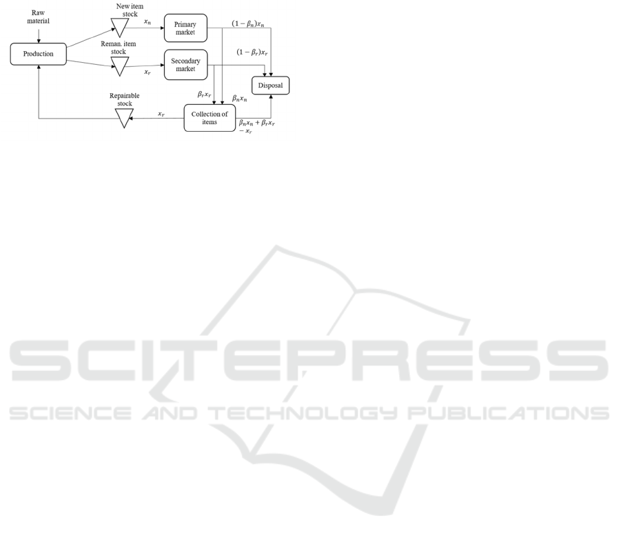
product flows that we consider is presented in Fig. 1
(detailed presentation of notations is provided after).
After being produced, new and remanufactured
products are placed in distinct inventories to serve
distinct markets. For the two types of products, after
a period of use, one part of the products sold is
directly disposed of while the other part can be
remanufactured and are collected. Not all collected
products are remanufactured and one part is disposed
of with respect to the decision of the number of
product that are remanufactured. Remanufactured
products are stored before being processed. The
systems thus contains three inventories with their
respective holding costs and two production
processes with their respective setup and unit cost.
a
https://orcid.org/0000-0001-8377-608X
b
https://orcid.org/0000-0003-0250-7959
We also consider price decisions for new and
remanufactured products and the problem is to
maximise a profit function including revenues from
the two markets, inventory holding and process costs.
As presented in Tang and Teunter (2006), for a
real case in automotive industry, remanufactured
products can be sold in the same market as new
products without distinction in price (as-good-as new
assumption). However, in many cases, they are sold
at lower prices. Most of the papers related to
inventory management for hybrid manufacturing /
remanufacturing systems consider as-good-as new
assumption. In this paper, we consider price decisions
and distinct markets for the two types of products as
in Godichaud and Amodeo (2022). Furthermore,
some customers may be undecided between the two
markets and can change according to selling prices.
This means that the products are in competition for a
common part of the two markets. This is modelled in
price-to-demand relationships. Constraints must be
added to the model to respect lower prices for
remanufactured products and the maximum part of
undecided customer between the markets.
In section 2, we present several works related to
our problem. The model with the notations and
assumptions are stated in section 3. Mathematical
146
Godichaud, M. and Amodeo, L.
Hybrid Manufacturing / Remanufacturing Inventory Model with Two Markets and Price Sensitive Demands with Competition.
DOI: 10.5220/0012429900003639
Paper published under CC license (CC BY-NC-ND 4.0)
In Proceedings of the 13th International Conference on Operations Research and Enterprise Systems (ICORES 2024), pages 146-157
ISBN: 978-989-758-681-1; ISSN: 2184-4372
Proceedings Copyright © 2024 by SCITEPRESS – Science and Technology Publications, Lda.
analysis and resolution method are developed in
section 4. A numerical example is presented in
section 5. Conclusion and extensions of this works are
summarized in section 6.
Figure 1: Material flows for hybrid systems with distinct
markets and competition.
2 RELATED WORKS
The problem of determining economic lot sizes has
long attracted the attention of researchers (Cárdenas-
Barrón et al., 2014; Andriolo et al. 2014). Recent
works tend to merge different features such as
financing practices, deterioration and shortage; see
e.g. in Tavakoli and Taleizadeh (2017), Taleizadeh et
al. (2020) for review and new models. Three research
streams in line with our problem have been identified:
inventory models with remanufacturing operations,
pricing and inventory-integrated models, pricing and
revenue management in reverse logistic with
remanufacturing.
In the field of inventory management with
returned and remanufactured products, there are
many papers and we restrict our attention on models
with EOQ/EPQ-like assumptions. The literature
review in (Bazan et al., 2016) highlights that there are
three clusters of models before the paper date based
on the models of (Richter, 1996), (El Saadany and
Jaber, 2008) and (Teunter, 2001). The works
reviewed in (Bazan et al., 2016) consider a single
market for new and remanufactured products. We
identified only two works that consider distinct
markets (Jaber and El Saadany, 2009; Hasanov et al.,
2012). They used an original assumption: the two
types of product are stored and sold separately over
distinct periods. This leads to stockout situation that
cannot be avoided. When one type of product is in
stock, demands for the other are backordered.
Several policies are investigated in literature that
considerer common production line for processing
different product types under EPQ assumptions, The
common cycle policies consist in having one EPQ
cycle for each product in one global cycle (Tang and
Teunter, 2006; Teunter et al., 2008; Teunter et al.,
2009; Nobil et al., 2020). They are easier to determine
but better results can be achieved by using basic
period policies (Zanoni et al., 2012), which consists
in determining cycle length for each product as
multiple of a basic period. For the case with only two
products, the basic period policy can be shown to be
optimal (Vemuganti, 1978). Basic approach to
determine optimal economic quantity is to derive the
related cost function. If this is simple enough without
constraint, closed-form equations can be obtained
even for the case with remanufacturing option. In the
case of multi-product ELS problem, the cost function
is more complex with specific constraints for the line
occupancy. Heuristics are then proposed in literature
(Teunter et al., 2009; Zanoni et al., 2012). We also
note that in all papers reviewed in this research stream
a cost function is used that contains setup and
inventory holding costs. More recently, Soleymanfa
et al. (2022) integrate sustainability related
parameters (environmental and social aspects) in the
cost function but consider same market for new and
returned products. (Hasanov et al. 2019) consider a
four level supply chain with energy, carbon emission
and disposal considerations. The literature review in
(Karim and Nakade, 2022) does not mentioned papers
assuming competition between new and
remanufactured products. In this paper, we consider
problems with two products, new and
remanufactured, but with price decisions and profit
objective function instead of a cost function.
Basis of models integrated pricing and EOQ/EPQ
are presented in Kunreuther and Richard (1971) for a
single item problem. The model can be extended to
consider multi-echelon serial supply chain (Lau &
Lau, 2003), wholesale price and discount policies
(Viswanathan and Wang, 2003) in the cases of single
market for one final product. The linear demand /
price function is commonly used because it facilitates
property analysis and is easy to adjust to field data.
The iso-elastic function presents the same advantages
in the cases without market competition (Ray et al.,
2005). In our work, we used linear demand function
with parameters modelling competition between
products, as in Bernstein and Federgruen (2003), and
we consider returned products and common
production line considerations with EPQ
assumptions. For the case where one production line
has to process several products, Salvietti and Smith
(2008) propose models and methods for ELS problem
with pricing decisions. The products are different and
sold on distinct market without competition. Our
work resumes the common line aspects but integrates
and analyses product returns and competition
Hybrid Manufacturing / Remanufacturing Inventory Model with Two Markets and Price Sensitive Demands with Competition
147

between products. In the context of reverse logistic,
Teksan and Geunes (2016) consider the coordination
between recovery decisions and selling prices for a
single product / market and the works of Pour-
Massahian-Tafti et al. (2020), Godichaud and
Amodeo (2020) address pricing problems in
disassembly systems. Relationship between price and
demand can be extended to consider perishable
product and promotion (Avinadav et al., 2016), stock
and shortage (Mishra et al., 2017). Taleizadeh et al.
(2019) consider pricing and EOQ integrated model
for substitutable products. In our work,
remanufactured and new products can be considered
as partially substitutable and additional constraints
are necessary. Taleizadeh et al. (2022) propose an
EOQ underlying wit partial credit, partial
backordering, carbon emissions and demand function
of selling price and carbon emissions. A signomial
geometric programming approach is proposed to
solve the problem. Finally, this paper extends
Godichaud and Amodeo (2022) by considering
competition between new and remanufactured
products, additional decision on inventory and further
analysis on decision process in this context.
Competition between products is considered in
several papers related to pricing / revenue
management in reverse logistic with
remanufacturing. Distinct markets with competition
for new and remanufacturing products are considered
in Majumder et al. (2001), Wu (2012), Wang et al.
(2019). Competition between different supply chain
agents is investigated in Ranjbar et al. (2020). We
note that linear relationship between demand and
price are used in all these papers. It facilitates model
analysis and derivation of closed-form equations for
optimal decision. Except in Guide et al. (2003), all
these works consider different agents for the recovery
of products and study roles of third party recover
partner in closed-loop supply chain. In the case of
two-echelon supply chain, wholesale prices are
considered as decision variables. Patoghi et al. (2022)
developed pricing model with different supply chain
actors with demands function of price, quality,
collection effort and return policy. The effect of
production constraints and inventory costs are
however not taken into account. We also note that in
these papers only simple unit proportional costs are
considered.
Based on the previous reviewed papers, we
propose in this paper an inventory model under EPQ
assumptions with manufacturing and
remanufacturing operations. Common production
line and return limitation constraints are considered.
Pricing decisions with two markets for newly
produced and remanufactured products is analysed.
3 MODEL STATEMENT
3.1 Notations
The material flows of the problem under study are
shown in Figure 1. The parameters, presented her
after, are related to the two processes, manufacturing
and remanufacturing, the three inventories (new,
remanufactured and repairable products) and the two
markets (primary for new products and secondary for
remanufactured products). The data and variables are
indexed by 𝑛 and 𝑟 for the new and remanufactured
items respectively.
Cost data are those of basic EPQ model for each
product stream (time unit is written in day but can be
changed depending on the context):
• 𝑠
, 𝑠
setup costs, [€/lot],
• ℎ
, ℎ
, ℎ
inventory holding costs( 𝑢 is for
returned products), [€/product.day],
• 𝑐
, 𝑐
unit production costs [€/product].
Process data and variables represent the two
processes with returned products and common line
utilization:
• 𝑚
, 𝑚
production rates [product/day],
• 𝜏
, 𝜏
setup times [day],
• 𝛽
, 𝛽
percentage of available items from primary
and secondary markets,
• 𝑡
, 𝑡
cycle lengths [day],
• 𝑏 basic period [day].
Demands or prices can be used as variables:
• 𝑥
, 𝑥
demand rates [product/day],
• 𝑦
, 𝑦
selling prices [€].
The relationships between demand rates and
selling prices are defined by the following
relationships:
• 𝑋
𝑦
,𝑦
=𝑑
−𝑎
𝑦
+𝑒𝑦
and 𝑋
𝑦
,𝑦
=
𝑑
−𝑎
𝑦
+𝑒𝑦
are the demand rates for new or
remanufactured items, each function of the selling
prices of the two types of items,
• 𝑌
𝑥
,𝑥
=𝑢
−𝑣
𝑥
−𝑤𝑥
and 𝑌
𝑥
,𝑥
=
𝑢
−𝑣
𝑥
−𝑤𝑥
are the unit selling prices of one
new or remanufactured item, function of the
demand rates of the two types of items.
For linear demand-to-price relationships, the
interpretation of the parameters is the following:
• 𝑑
, 𝑑
maximum demands for new items and
remanufactured items (markets size),
• 𝑎
, 𝑎
, 𝑒 price to demand function parameters
(linear relationships),
ICORES 2024 - 13th International Conference on Operations Research and Enterprise Systems
148

• 𝑢
, 𝑢
maximum prices,
• 𝑣
, 𝑣
, 𝑤 demand to price function parameters.
The same competition parameter, 𝑒, is used is the
two functions, 𝑋
and 𝑋
, based on the following
interpretation of the competition. There are some
undecided customers between buying a new product
or a remanufactured product. Their decision is made
based on the price difference 𝑦
−𝑦
. For a given
price difference, 𝑒
𝑦
−𝑦
represents the number of
customers (per unit of time) that change their willing
to buy a new product to buy a remanufactured one.
Initially, the functions 𝑋
and 𝑋
can be defined by
𝑋
𝑦
,𝑦
=𝑑
−𝑎
𝑦
−𝑒
𝑦
−𝑦
and
𝑋
𝑦
,𝑦
=𝑑
−𝑎′
𝑦
+𝑒
𝑦
−𝑦
. By setting
𝑎
=𝑎
+𝑒 and 𝑎
=𝑎′
+𝑒, we retrieve the
previous function. We also note that given this
interpretation of the competition, we impose
constraint 𝑦
>𝑦
, otherwise undecided customer
prefer to buy a new product. The change between
demand functions and price functions can be done
using the following relationships:
𝑣
=𝑎
𝑎
𝑎
−𝑒
⁄
, 𝑢
=𝑣
𝑑
+𝑑
𝑒𝑎
⁄
,
𝑤=𝑣
𝑒𝑎
⁄
=𝑣
𝑒𝑎
⁄
, 𝑣
=𝑎
𝑎
𝑎
−𝑒
⁄
,
𝑢
=𝑣
𝑑
+𝑑
𝑒𝑎
⁄
.
3.2 Assumptions
The problem assumptions follow those of traditional
EPQ and ELS-R with remanufactured returns:
• Demands, production and returns are
characterized by rates (items per day for instance),
and they are constant,
• Inventory are continuously reviewed (continuous
time inventory model),
• Cost and profit indicators are defined in average
(unit of money per unit of time) on an infinite time
horizon,
• There is a fixed cost incurred for each production
setup (before starting a production lot) and one
unit in inventory per unit of time generates an
holding cost,
• Backlogs or lost sales are not allowed in this work.
In addition to the previous presentation of
relationship between prices and demands, we add the
following assumptions more specific to the problem
under study:
• There are two markets, one for new products and
one for remanufactured products, but one
production line to produce the two types of
products,
• Production rate, holding and setup costs are
different for the two types of product,
• Demands or prices for the two markets are set
once at the beginning of the planning horizon,
• Only the returned products that will be
remanufactured are kept in the return inventory, if
the returns are superior to the remanufacturing
quantity, the surplus is disposed of (i.e. directed to
others recovery channels).
These assumptions justify the rate associated to
the material flows in Figure 1. The products
availability from the production line must be 𝑥
and
𝑥
to satisfy demands in each markets. After the
period of use, 𝛽
𝑥
+𝛽
𝑥
products are available for
remanufacturing. However, only 𝑥
are
remanufactured and 𝛽
𝑥
+𝛽
𝑥
−𝑥
are disposed
of. The return inventory is replenished continuously
at rate 𝑥
.
Based on previous assumptions, the evolution of
the three inventories over time is presented in Figure
2. The curves In, Ir and Iu represent respectively the
new, remanufactured and repairable product
inventories. Curve shapes are basic saw tooth profiles
due to EPQ-related assumptions. There is a repetition
of two phases for each inventory: one production-
consumption phase and one consumption-only phase.
For In and Ir, inventories first increase at rate 𝑚
−
𝑥
and 𝑚
−𝑥
and then decrease at rate 𝑥
and 𝑥
.
The duration of the two phases is 𝑡
(resp. 𝑡
) and the
first lasts
𝑥
𝑚
⁄
𝑡
(resp.
𝑥
𝑚
⁄
𝑡
. For Iu,
inventory first increases at rate 𝑥
and then decrease
at rate 𝑚
−𝑥
symmetrically to inventory Ir. Only
the returned products that will be remanufactured are
kept in the return inventory and there is only a
common setup cost to move an item between the two
inventories with remanufacturing process.
The low part (under the graph) of Figure 2 shows
the production line occupancy. There is one repetitive
cycle with two new production lot, one
remanufacturing lot and idle time between lots in this
example. Setup times take place before each lot.
Basic period policy is used to ensure that the
solution defining the cycle length of each product is
feasible without overlapping. Basic period policy has
the following characteristics:
• The cycle length of each type of product is an
integer multiple of the basic period,
• One basic period can contain one production
phase and one setup for each type of product.
Hybrid Manufacturing / Remanufacturing Inventory Model with Two Markets and Price Sensitive Demands with Competition
149
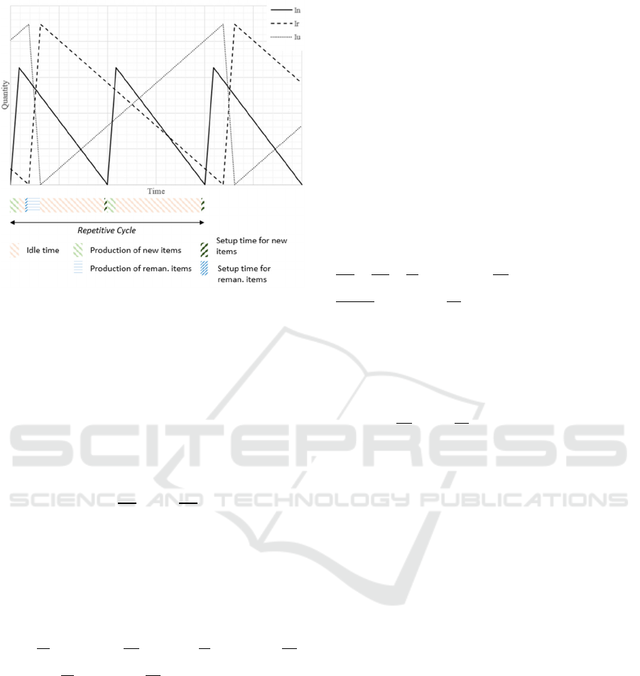
Figure 2: Inventories evolution over time.
Based on the results in (Vemuganti, 1978), basic
period policy is optimal for two products if the basic
period is a variable. In Figure 2, the repetitive cycle
lasts two basic periods with two new product batches
and one remanufacturing batch. The first basic period
in the cycle contains the productions and setup times
for one cycle of each type of products. By denoting
with 𝑏 the length of the basic period and 𝑘
, 𝑘
the
integer multiples, the basic period impose that 𝑡
=
𝑘
𝑏 and 𝑡
=𝑘
𝑏 and the following constraint:
𝜏
+𝜏
+
𝑥
𝑚
𝑘
𝑏+
𝑥
𝑚
𝑘
𝑏𝑏
According to the previous assumptions, especially
constant demand, production and return rates and
continuous time review, one can note that on Figure
2 that inventories are linear functions of time.
Average inventory holding cost for the three
inventories, denoted by 𝐻
, 𝐻
and 𝐻
([€/day]) are
given by, setting 𝑡
=𝑘
𝑏 and 𝑡
=𝑘
𝑏:
𝐻
=
𝑘
𝑏𝑥
1−
, 𝐻
=
𝑘
𝑏𝑥
1−
and 𝐻
=
𝑘
𝑏𝑥
1−
.
As mentioned previously, we consider
competition as a part of consumers, positioned
between the two markets, which are sensitive to the
price difference between the two products.
Furthermore, we also consider that if the
remanufactured product price is higher than the new
product price then no customer will want to buy a
remanufactured product. The constraint 𝑌
≥𝑌
is
then added to the model.
The parameter 𝑑
being interpreted as the
remanufactured product market size, the constraint
𝑑
−𝑎
−𝑒𝑌
≥0 is necessary. Mathematically,
without this constraint, it is possible to have 𝑥
=
𝑑
−𝑎
𝑌
+𝑒𝑌
>0 and 𝑑
−𝑎
−𝑒𝑌
0.
Constraint 𝑑
−𝑎
−𝑏𝑌
≥0 is not necessary
since we must have 𝑥
=𝑑
−
𝑎
−𝑒
𝑌
−𝑒
𝑌
−
𝑌
≥0 and 𝑌
≥𝑌
.
3.3 Model
The problem is to maximise the system average
profit, denoted by 𝛱
𝑥
,𝑥
,𝑘
,𝑘
,𝑏
, with the
decision variables 𝑥
, 𝑥
, 𝑘
, 𝑘
and 𝑏 under the
previous assumptions. The resulting model is a non-
linear mixed integer program with constraints defined
by (1)-(5).
𝛱
𝑥
,𝑥
,𝑘
,𝑘
,𝑏
=
𝑌
−𝑐
𝑥
+
𝑌
−𝑐
𝑥
−
−
−
𝑘
𝑏𝑥
1−
−
𝑘
𝑏𝑥
1−
(1)
−𝛽
𝑥
−
𝛽
−1
𝑥
0 (2)
−𝑣
+𝑤
𝑥
+
𝑣
−𝑤
𝑥
𝑢
−𝑢
(3)
−𝑣
𝑥
−𝑤𝑥
𝑤
𝑣
−𝑤
⁄
𝑢
−𝑢
(4)
𝜏
+𝜏
+
𝑘
𝑏+
𝑘
𝑏𝑏 (5)
The first two terms of the objective function
represent profit without inventory related parameters.
We denote it by 𝑀
𝑥
,𝑥
. The following two terms
are the average setup costs and the last two are the
average holding costs. The objective function is
different from (Godichaud & Amodeo, 2022) with
consideration of competition (different 𝑌
and 𝑌
functions) and 𝑏 as decision variable. Constraints (2)
to (5) arise from previous assumptions. Constraint (2)
limits the available returns for remanufacturing.
Constraint (3) corresponds to 𝑌
≥𝑌
with respect to
decisions variable 𝑥
and 𝑥
. Constraint (4) forces
𝑑
−𝑎
−𝑒𝑌
≥0. Constraint (5) is the basic
period policy constraint.
4 MATHEMATICAL ANALYSIS
AND RESOLUTION
APPROACHES
The problem models by (1)-(5) is a non-linear
programming model (objective function and
constraint (5) are non-linear) with integer variables
𝑘
and 𝑘
. We propose to decompose its analysis into
sub-problems having good properties for solving and
analysis of solutions. The problem without inventory
ICORES 2024 - 13th International Conference on Operations Research and Enterprise Systems
150

related costs is first studied to obtain an initial
solution (section 4.1). This solution is completed
sequentially with the determination of inventory
related variables with respect to a 2-items ELS
problem (section 4.2). The solution is then iteratively
improved with non-linear resolution methods.
This decomposition enables to compare three
resolution approaches:
• Sequential resolution: this approach use the
properties of the pricing presented section 4.1 and
ELS resolution method.
• One iteration resolution: it adds one step to adjust
the demands based on the cycle lengths find in the
sequential resolution. This is a modified pricing
problem integrating inventory-holding costs
presented in section 4.3.
• Joint optimisation: based on the initial solution
found with the one iteration resolution, all the
variables are optimised simultaneously based on
the procedure presented in section 4.3.
4.1 Problem Without Inventory
Related Costs
We consider only the first two terms of the profit
function (1). It reduces to the profit function denoted
by 𝑀
𝑥
,𝑥
, with only variables 𝑥
and 𝑥
, which is
a sum of common functions in pricing problems.
There are two motivations to study this sub-problem
apart. In many companies, as mentioned in
(Kunreuther and Richard, 1971), a sequential
decision process is performed. Prices are decided
first, by marketing department, and then, production
and inventory decisions are made with the demands
associated with the given prices. In our case, 𝑘
, 𝑘
and 𝑏 would be decided in a second step with 𝑥
, 𝑥
fixed in a first step. Even in case where integrated
decisions are made, solving sub-problem without
inventory related costs gives initial values.
Replacing 𝑌
and 𝑌
as function of 𝑥
and 𝑥
,
𝑀
𝑥
,𝑥
is quadratic function:
𝑀
𝑥
,𝑥
=
𝑢
−𝑣
𝑥
−𝑤𝑥
−𝑐
𝑥
+
𝑢
−𝑣
𝑥
−𝑤𝑥
−𝑐
𝑥
Its stationary points are:
𝑥̅
=
and 𝑥̅
=
𝑀
𝑥
,𝑥
is concave for 𝑥
>0 and 𝑥
>0.The
constraints (2)-(4) are linear and the sub-problem of
maximising 𝑀
𝑥
,𝑥
w.r.t. (2)-(4) is solve rapidly
with a solver or feasible direction methods.
4.2 Initial EPQ Problem with Two
Products and a Common Line
If 𝑥
and 𝑥
are fixed, the problem reduces to the
minimisation of inventory related cost (setup and
holding) subject to constraint (5). Furthermore, for
given value of 𝑘
and 𝑘
, the optimal value for 𝑏 is:
𝑏
=
⁄
⁄
(6)
Constraint (5) gives the minimal value for 𝑏,
denoted by 𝑏
, to process the two types of products
on the same production line without overlapping of
production runs:
𝑏
=
𝜏
+𝜏
1 −
+
(7)
The solution of the problem, for given values of
𝑥
, 𝑥
, 𝑘
and 𝑘
, are then 𝑏=𝑚𝑎𝑥𝑏
,𝑏
.
The value for 𝑘
and 𝑘
are tested iteratively in the
overall procedure.
4.3 Joint Optimisation
Previous sub-problem can be extended with
inventory-related decision variables (𝑘
, 𝑘
and 𝑏)
fixed (setup costs are constant but holding cost vary
w.r.t. 𝑥
and 𝑥
). The objective function then remains
quadratic and concave (under the following
conditions) with one stationary point given directly
by the following equations:
𝑥
=
𝑣
𝑢
−𝑐
−𝑤
𝑢
−𝑐
2
𝑣
𝑣
−𝑤
,
𝑥
=
𝑣
𝑢
−𝑐
−𝑤
𝑢
−𝑐
2
𝑣
𝑣
−𝑤
with 𝑐
=𝑐
+ℎ
𝑘
𝑏2
⁄
, 𝑐
=𝑐
+
ℎ
+ℎ
𝑘
𝑏2
⁄
, 𝑣
=2𝑣
−ℎ
𝑘
𝑏𝑚
⁄
and 𝑣
=
2𝑣
−
ℎ
+ℎ
𝑘
𝑏𝑚
⁄
. The function is concave for
4𝑣
𝑣
−4𝑤
>0.
With 𝑘
, 𝑘
and 𝑏 fixed, constraint (5) is linear as
constraint (2)-(4). Based on the previous properties,
this sub problem can be solved by using any feasible
direction methods.
At a second level, 𝑘
, 𝑘
are fixed and a line
search is applied with respect to 𝑏. Based on initial
values of 𝑥
, 𝑥
, the first value of 𝑏 for the line search
is determined. Values of 𝑥
, 𝑥
are then determined
for each value of 𝑏 by solving the problem with 𝑘
,
𝑘
and 𝑏 fixed. Numerically, based on instances we
used, the search of 𝑏 with built-in optimisation on 𝑥
,
𝑥
gives concave profit function.
Hybrid Manufacturing / Remanufacturing Inventory Model with Two Markets and Price Sensitive Demands with Competition
151

At a higher level, values of 𝑘
, 𝑘
are examined
with nested iterations. Starting with 𝑘
=𝑘
=1, the
values are increased while the profit function
increases. The following procedure can be used to
solve the overall problem, we denote by 𝜋
∗
the best
profit found during the procedure with 𝑘
∗
, 𝑘
∗
, 𝑥
∗
, 𝑥
∗
and 𝑏
∗
the related decisions:
• Step1. Solve the problem without inventory
related cost (section 4.1) to have initial value for
𝑥
, 𝑥
. Set 𝑘
=𝑘
=𝑘
∗
=𝑘
∗
=1, 𝑥
∗
=𝑥
,
𝑥
∗
=𝑥
and 𝑏
∗
=𝑏=𝑚𝑎𝑥𝑏
,𝑏
and
compute the first best profit 𝜋
∗
.
• Step 2. Set 𝑏=𝑚𝑎𝑥𝑏
,𝑏
. Adjust value
for 𝑥
, 𝑥
with inventory related cost with 𝑏
fixed.
• Step 3. Apply line search on 𝑏 with built-in
optimisation on 𝑥
, 𝑥
and compute the profit,
denoted by 𝜋
, for the obtained value. If 𝜋
>𝜋
∗
,
update the best solution (set 𝜋
∗
=𝜋
and 𝑘
∗
, 𝑘
∗
,
𝑥
∗
, 𝑥
∗
and 𝑏
∗
to the current value of 𝑘
, 𝑘
, 𝑥
,
𝑥
and 𝑏), set 𝑘
←𝑘
+1 and go back to Step 2,
else if 𝑘
=𝑘
∗
, set 𝑘
←𝑘
+1 and go back to
Step 2, else go to Step 4.
• Step 4. Return the best solution found.
5 NUMERICAL ANALYSIS
A first set of instances is generated based on the
instance generator proposed in Salvietti and Smith
(2008). The following steps are used to generate
instances (𝑈[𝑙𝑜𝑤𝑒𝑟 𝑢𝑝𝑝𝑒𝑟] corresponds to uniform
distribution between specified lower and upper value
of the parameters). The time unit is one day.
• Market sizes are generated with 𝑑
=
𝑈[4000 5000] and 𝑑
=𝑈[0.2 0.8] × 𝑑
(we
study cases where secondary market is smaller
than primary market).
• Maximum price are generated with 𝑌
,
=
𝑈[20 50] and 𝑌
,
=𝑈[0.5 0.8] × 𝑌
,
(the
maximum price of remanufactured products is
lower since we assume this constraint in the
model).
• To generate values for 𝑒 (competition parameter),
we used a maximum market change parameter,
denoted here by 𝑋
(defined for instance
generation only). It represents the percentage of
customers who can change from new to
remanufactured products. We used 𝑋
=
𝑈[0.05 0.2] × 𝑑
and 𝑒=𝑋
𝑌
,
⁄
.
• Price-to-demand parameter are deduced from
previous parameters with: 𝑎
=𝑑
𝑌
,
⁄
+𝑒
and 𝑎
=𝑑
𝑌
,
⁄
+𝑒.
• Unit cost are generated with 𝑐
=𝑈[0.1 0.5] ×
𝑢
, to avoid infeasible instances with 𝑐
>𝑢
,
and 𝑐
=𝑈[0.2 0.9] × 𝑐
.
• Based on (Salvietti et al., 2008), set-up and
inventory holding costs are generated with 𝑠
=
𝑈[30 50] , 𝑠
=𝑈[30 50] , ℎ
=
𝑈[0.05 0.1] × 𝑐
100
⁄
, ℎ
=
𝑈[0.05 0.1] × 𝑐
100
⁄
and ℎ
=𝑈[0.1 0.5] ×
ℎ
; production rates with 𝑚
=𝑈[2000 4000]
and 𝑚
=𝑈[2000 4000]; set-up times with 𝑡
=
𝑈[0.05 0.3] and 𝑡
=𝑈[0.05 0.3].
These instances can be considered as high-level
demands and low-level inventory costs. Table 1
presents data for three instances from this dataset.
Instance 0 is obtained with median values of the
distribution ranges. We generated more than one
thousand instances and the instance 1 and 2 in Table
1 correspond to those that give the best and the worst
profit respectively.
The first part of Table 2 presents values of
decision variables and profit for instances in Table 1
with the three decision processes presented in section
4.
Table 1: Instances generated based on (Salvietti and Smith,
2008).
Ins.
Data
0
𝑑
=4500 𝑎
=144.63 𝑑
=2250 𝑎
=114.96
𝑒=16.06 𝑐
=10.14 𝑐
=5.58 𝑠
=40 𝑠
=40
ℎ
=7.61E-03 ℎ
=4.2E-03 𝑚
=3000 𝑚
=3000
𝜏
=0.175 𝜏
=0.175 𝛽
=0.667 𝛽
=0.667
1
𝑑
=4948 𝑎
=121.65 𝑑
=3859 𝑎
=142.25
𝑒=18.56 𝑐
=4.74 𝑐
= 3.62 𝑠
=45.1 𝑠
=46.6
ℎ
=4.09E-03 ℎ
=4.07E-03 𝑚
=3742
𝑚
=2747 𝜏
=0.21 𝜏
=0.29 𝛽
=0.667 𝛽
=0.667
2
𝑑
=4016 𝑎
=238.95 𝑑
=1767 𝑎
=180.65
𝑒=38.15 𝑐
=9.07 𝑐
= 7.22 𝑠
=30.13 𝑠
=49.04
ℎ
=4.58E-03 ℎ
=5.22E-03 𝑚
=3400
𝑚
=2409 𝜏
=0.13 𝜏
=0.16 𝛽
=0.667 𝛽
=0.667
In this type of instances, inventory related cost
(setup + holding costs) are very small compared to
unit proportional costs (𝑐
𝑥
+𝑐
𝑥
). One can note
that inventory costs have little effect on the overall
profit. The variation of decisions and profit are then
small between the three decision processes. In this
case, a sequential decision process in two phases is
sufficient while having properties of separate models
presented in section 4. One limitation is that demands
values generated in the first phase can be infeasible
for the second phase if 𝑥
𝑚
⁄
+𝑥
𝑚
⁄
≥1. This is
ICORES 2024 - 13th International Conference on Operations Research and Enterprise Systems
152
observed in 23% of the instances generated. This
limitation can be solved by introducing a constraint
𝑥
𝑚
⁄
+𝑥
𝑚
⁄
<𝛼, with 𝛼<1, in the problem of
the first phase. It also allows having an initial solution
for the joint optimization problem. This is the case of
instance 1.
In instance 0, basic period constraint is not
binding (line occupancy is 0.895 < 1) with the optimal
demands. The line occupancy is equal to one in all
instances where the first phase of the sequential
decisions give infeasible for the second phase. The
basic period constraint has a greater effect when the
second market demand is small compared to primary
market demand when it is not possible to place two or
more remanufacturing lot with one manufacturing lot
in one basic period.
In instance 2, we note again no significant
variation of variables and profit between the three
decision processes and the inventory cost represents
a small parts of the overall cost. In this instance, two
remanufacturing lot can be optimally placed in one
basic period for one manufacturing lot. In instance 1,
the first phase of the sequential decision gives
infeasible solutions. We add the constraint mentioned
before to obtain an initial solution for the joint
optimisation.
The lines “Stat.” in Table 2 presents the means
and standard deviations of variables and indicators
over 1200 instances generated. We note significant
variation of the basic period length ( 𝑏) due to
constraint (5). The constraint is saturated in 34% of
instances and, for these ones, the basic period and
inventory costs tend to be larger. We also note that
only 53% of the returned products are
remanufactured. If environmental constraints impose
higher remanufacturing rate, the producer have to
accept lower profit.
Table 2: Results for instances generated based on (Salvietti
and Smith, 2008).
Ins. Results (decisions and profit)
0
Joint
𝑘
=1 𝑘
=1 𝑏=4.39 Profit=26728.76
𝑥
=1561.35 𝑥
=885.55 𝑦
=21.98
𝑦
=14.94
Sequ
𝑘
=1 𝑘
=1 𝑏=4.39 Profit=26728.76
𝑥
=1561.27 𝑥
=885.77 𝑦
=21.98
𝑦
=14.94
1-
iter
𝑘
=1 𝑘
=1 𝑏=53.07 Profit=68440.76
𝑥
=1975.60 𝑥
=885.77 𝑦
=21.98
𝑦
=14.94
1
Joint
𝑘
=1 𝑘
=1 𝑏=4.39 Profit=26728.76
𝑥
=1561.35 𝑥
=1271.53 𝑦
=27.76
𝑦
=21.81
Sequ
Profit=70770.01 𝑥
=2219.3
𝑥
=1716.02 𝑦
=25.23 𝑦
=18.36 (not
feasible w.r.t.
(
5
))
2
Joint
𝑘
=1 𝑘
=2 𝑏=3.99 Profit=6580.4
𝑥
=1061.94 𝑥
=403.18 𝑦
=14.04
𝑦
=10.51
Sequ
𝑘
=1 𝑘
=2 𝑏=3.99 Profit=6580.4
𝑥
=1062.08 𝑥
=404.36 𝑦
=14.04
𝑦
=10.51
1-iter
𝑘
=1 𝑘
=2 𝑏=3.99 Profit=6580.4
𝑥
=1061.94 𝑥
=403.18 𝑦
=14.04
𝑦
=10.51
Stat. Joint
b=11.88(15.58)
Profit=26940.97(11003.8) 𝑥
=1497.0
(248.12) 𝑥
=842.78(301.76)
𝑦
=22.45(5.81) 𝑦
=15.32 (4.29)
Joint = joint optimisation of all variables, Sequ =
demand variables first and reorder interval variables
after, 1-iter = reorder interval variables fixed by Sequ
and re-optimisation of demand variables, line Stat gives
mean value and standard deviation over 1200 instances.
0 Joint
InvCost=36.48 LineOcc=0.895
Return=1631.27 Rem./Return=0.543
Market change=113.015
1 Joint
InvCost=176.86 LineOcc=1
Return=2164.77 Rem./Return=0.59
Market chan
g
e=110.46
2 Joint
InvCost=27.36 LineOcc=0.72
Return=976.75 Rem./Return=0.41
Market chan
g
e=134.54
Stat Joint
InvCost=48.22 (25.12) LineOcc=0.90
(0.10) Return=1559.90 (276.5)
Rem./Return=0.53
(0.13) Market change=111.82
(
46.72
)
InvCost = order + holding costs, LineOcc = setup +
production times on basic period length, Return = return
rate of products that can be remanufactured,
Rem./Return = proportion of remanufacturable products
which are actually remanufactured, Market change =
part of secondary market that comes from primary
market.
Hybrid Manufacturing / Remanufacturing Inventory Model with Two Markets and Price Sensitive Demands with Competition
153
In the previous dataset, the joint optimisation
brings no profit improvement or change in variables
values. This is due to the low level of inventory-
related costs (setup plus holding costs) compared to
that of proportional costs (𝑐
𝑥
+𝑐
𝑥
). In this type
of instance the sequential resolution, give solutions
closed to optimum and cycle lengths variation does
not lead to significant profit variation. We observe
this fact, in all dataset form ELS-related literature we
have tested (questioning the importance of
sophisticated method compared to simple ones like
common cycle policy). A second set of examples is
generated to analyse others types of practical
situations. These examples are adapted from
literature. The data are presented in Table 3 and the
results are presented in Table 4. These examples have
lower market sizes (which must lead to lower
demands and production volumes) and higher
inventory holding costs (the gap between inventory-
related costs and proportional costs increases with
respect to the demand). The time unit is one day.
Table 3: Additional instances based on literature on EOQ-
pricing and ELS problems.
Ins. Data
5
𝑑
=40 𝑎
=1.608 𝑑
=32 𝑎
=2.568 𝑒=0.32
𝑐
=10 𝑐
=5 𝑠
=50 𝑠
=50 ℎ
=1 ℎ
=0.85
𝑚
=50 𝑚
=30 𝜏
=0.5 𝜏
=0.5 𝛽
=0.67
𝛽
=0.67
6
𝑑
=40 𝑎
=1.608 𝑑
=32 𝑎
=2.568 𝑒=0.32
𝑐
=10 𝑐
=5 𝑠
=50 𝑠
=50 ℎ
=1 ℎ
=0.85
𝑚
=50 𝑚
=30 𝜏
=2 𝜏
=2 𝛽
=0.67 𝛽
=0.67
7
𝑑
=100 𝑎
=0.334 𝑑
=80 𝑎
=0.534 𝑒=0.067
𝑐
=15 𝑐
=13 𝑠
=150 𝑠
=150 ℎ
=4.5 ℎ
=4.1
𝑚
=100 𝑚
=100 𝜏
=0.5 𝜏
=0.5 𝛽
=0.67
𝛽
=0.67
8
𝑑
=100 𝑎
=2.004 𝑑
=80 𝑎
=3.34 𝑒=0.4 𝑐
=15
𝑐
=13 𝑠
=150 𝑠
=150 ℎ
=4.5 ℎ
=4.1 𝑚
=100
𝑚
=100 𝜏
=0.5 𝜏
=0.5 𝛽
=0.67 𝛽
=0.67
9
𝑑
=100 𝑎
=3.34 𝑑
=80 𝑎
=3.204 𝑒=0.67
𝑐
=15 𝑐
=13 𝑠
=150 𝑠
=150 ℎ
=4.5 ℎ
=4.1
𝑚
=100 𝑚
=100 𝜏
=0.5 𝜏
=0.5 𝛽
=0.67
𝛽
=0.67
10
𝑑
=20 𝑎
=0.404 𝑑
=16 𝑎
=0.404 𝑒=0.08
𝑐
=25 𝑐
=20 𝑠
=130 𝑠
=130 ℎ
=1.2 ℎ
=0.85
𝑚
=100 𝑚
=100 𝜏
=0.5 𝜏
=0.5 𝛽
=0.67
𝛽
=0.67
Instances 5 and 6 are generated as the previous
one except that the market size is 40 (products per
day) instead of 4000. The difference between the two
are the setup times (0.5 and 2 days) to get insights on
the effect of constraint (5) and the utilisation of a
common production line. For instance 5, inventory-
related costs represents 24% of the total costs for the
sequential solution (we remind that it is also the initial
solution for the joint solution) which is significant.
However, the variation in profit and decision
variables is not. The line occupancy in less than 1
allowing the basic period length 𝑏 to be at the
optimum and the inventory cost function is flat at this
value. On the contrary, in instance 6, the setup times
are long, 2 days while the basic period length is 7.52
days, and the constraint (5) is saturated. A gap of
24.5% is observed between the sequential and joint
methods while the inventory-related costs represents
29% of the total costs for the sequential solution close
to instance 5. In this case, the joint method act
simultaneously on the basic period length and the
demands to find the optimal values along the
constraint. In these two instances, more returned
products are used in proportion compared to first
dataset, but not all.
Instances 7 to 9 are adapted from (Taleizadeh et
al. 2019), who study a real case application of pricing-
inventory model for two substitutable products.
Instance 7 have high maximum prices compared to
unit costs. We also note that the inventory holding
costs are very high, assuming the integration of more
aspects than the financing part (warehousing, energy,
handling resources …). Instances 8 and 9 are
generated from instance 7 by reducing the maximum
prices in order to have a greater share of inventory
cost in the profit and analyse the behaviour of the
resolution methods in these cases. For the three
instances, inventory-related costs represents around
30% of the total costs for the sequential solution but
the variation in the profit is limited: 1.4%, 1.3% and
3.7% for instances 7, 8 and 9 respectively. In instance
7, the variation in inventory-related costs is 30%
between sequential and joint solutions showing the
simultaneous effect of cycle length and demands.
These results also show the quality of the sequential
solution as initial solution for the joint resolution. The
remanufacturing rate is close to that obtained from the
first dataset and remains low (half of the return
product are remanufactured).
Instance 10 is adapted from (Zipkin, 2000) and
has higher setup and holding costs and low demands.
The time basis is the week. The inventory-related
costs represents 24% of the total costs but the
variation of the profit is again limited to 1.7%
between sequential and joint solutions. Constraint (5)
is not saturated and the percentage of returned
products that are remanufactured is higher than in the
first dataset.
ICORES 2024 - 13th International Conference on Operations Research and Enterprise Systems
154
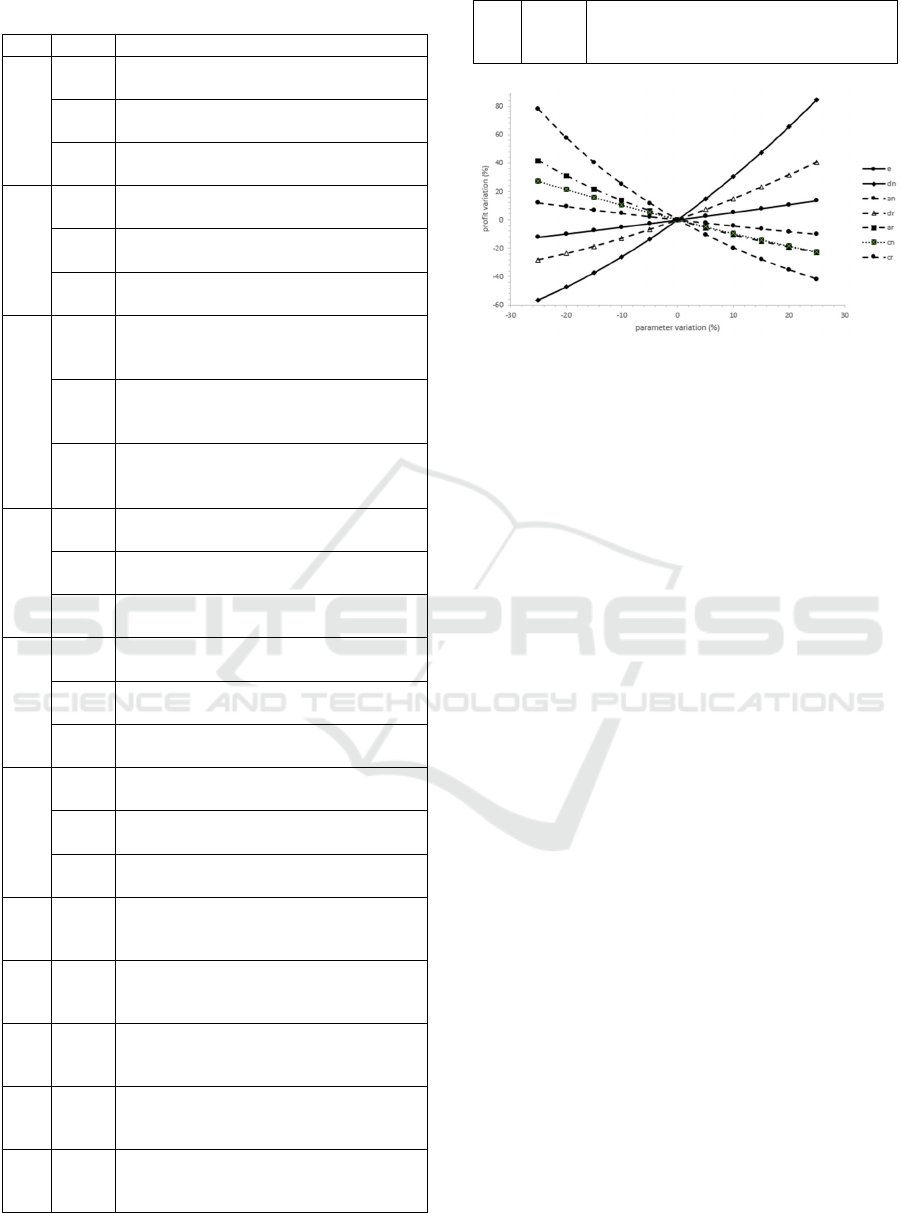
Table 4: Results for the second set of instances.
Ins. Results
(
decisions and
p
rofit
)
5
Joint
𝑘
=1 𝑘
=1 𝑏=3.65 Profit=121.18
𝑥
=12.07 𝑥
=10.77 𝑦
=19.5 𝑦
=10.7
Sequ
𝑘
=1 𝑘
=1 𝑏=3.60 Profit=120.8
𝑥
=12.76 𝑥
=11.18 𝑦
=19.01 𝑦
=10.48
1-iter
𝑘
=1 𝑘
=1 𝑏=3.60 Profit=121.17
𝑥
=12.08 𝑥
=10.78 𝑦
=19.49 𝑦
=10.69
6
Joint
𝑘
=1 𝑘
=1 𝑏=7.25 Profit=104.6
𝑥
=10.71 𝑥
=7.02 𝑦
=20.66 𝑦
=12.3
Sequ
𝑘
=1 𝑘
=1 𝑏=10.75 Profit=83.99
𝑥
=12.76 𝑥
=11.18 𝑦
=19.03 𝑦
=10.48
1-iter
𝑘
=1 𝑘
=1 𝑏=10.75 Profit=87.89
𝑥
=10.52 𝑥
=9.54 𝑦
=20.58 𝑦
=11.31
7
Joint
𝑘
=1 𝑘
=1 𝑏=4.49 Profit=10457.68
𝑥
=45.58 𝑥
=32.15 𝑦
=185.44
𝑦
=112.76
Sequ
𝑘
=1 𝑘
=1 𝑏=6.65 Profit=10311.15
𝑥
=47.93 𝑥
=36.03 𝑦
=176.36
𝑦
=102.49
1-iter
𝑘
=1 𝑘
=1 𝑏=6.65 Profit=10312.90
𝑥
=47.95 𝑥
=37.03 𝑦
=176.67
𝑦
=104.39
8
Joint
𝑘
=1 𝑘
=1 𝑏=2.13 Profit=662.51
𝑥
=36.29 𝑥
=16.84 𝑦
=36.64 𝑦
=24.29
Sequ
𝑘
=1 𝑘
=1 𝑏=2.48 Profit=646.43
𝑥
=37.57 𝑥
=22.17 𝑦
=35.64 𝑦
=22.50
1-iter
𝑘
=1 𝑘
=1 𝑏=2.48 Profit=654.18
𝑥
=36.76 𝑥
=17.1 𝑦
=36.38 𝑦
=24.17
9
Joint
𝑘
=1 𝑘
=1 𝑏=1.98 Profit=211.27
𝑥
=26.62 𝑥
=19.91 𝑦
=26.62 𝑦
=23.31
Sequ
𝑘
=1 𝑘
=1 𝑏=2.11 Profit=203.68
𝑥
=29.28 𝑥
=23.29 𝑦
=25.58 𝑦
=22.08
1-iter
𝑘
=1 𝑘
=1 𝑏=2.11 Profit=210.69
𝑥
=26.42 𝑥
=19.65 𝑦
=26.7 𝑦
=23.4
10
Joint
𝑘
=3 𝑘
=4 𝑏=2.18 Profit=106.04
𝑥
=5.18 𝑥
=4.42 𝑦
=44.1 𝑦
=37.4
Sequ
𝑘
=3 𝑘
=4 𝑏=2.07 Profit=104.24
𝑥
=5.75 𝑥
=4.96 𝑦
=42.34 𝑦
=35.71
1-iter
𝑘
=3 𝑘
=4 𝑏=2.07 Profit=105.95
𝑥
=5.21 𝑥
=4.45 𝑦
=44.01 𝑦
=37.31
5 Joint
InvCost=54.82 LineOcc=0.87
Return=15.23 Rem./Return=0.71
Market chan
g
e =2.82
6 Joint
InvCost=60.86 LineOcc=1
Return=11.82 Rem./Return=0.59
Market chan
g
e =2.68
7 Joint
InvCost=518.19 LineOcc=1
Return=51.82 Rem./Return=0.62
Market chan
g
e =4.85
8 Joint
InvCost=312.85 LineOcc=1
Return=35.42 Rem./Return=0.48
Market change =4.94
9 Joint
InvCost=303.25 LineOcc=0.97
Return=31.02 Rem./Return=0.64
Market change =2.21
10 Joint
InvCost=69.7 LineOcc=0.79
Return=6.4 Rem./Return=0.69 Market
change =54
Figure 3: Sensitivity analysis for instance 5.
Figure 3 presents the result of a sensitivity
analysis on instance 5. We focus on demand function
parameters and unit process costs (𝑐
and 𝑐
) as we
had seen that inventory related had small effect on the
profit over all instances. Each parameter is varied one
at a time keeping all other parameters constant, from
-25% to 25% by step of 5%. The profit is determined
with the joint optimisation for each value. We first
note that the profit is more sensitive to parameters 𝑑
and 𝑎
(primary market) with opposite direction. The
profit increased with respect to 𝑒 but with smaller
amplitude as it concerns less customers. As expected,
if the unit process costs increased, the profit
decreased. We perform the same analysis on
parameter 𝛽
and 𝛽
but no variation in the profit and
decision variables is observed. As constraint (2) is not
saturated, 𝑥
is constant and the proportion of
returned product that are remanufactured simply
decreased as 𝛽
or 𝛽
increased. We performed the
same analysis in the other instances and the same
trends are observed but with different amplitudes.
6 CONCLUSION
In many real situations, remanufacturing offers the
opportunity to sell product at lower price when some
customers want to pay less for a remanufactured
product while the others prefer to buy new one at
higher price. We have developed a new model for
hybrid system that produces new and remanufactured
products for two distinct markets. We have modelled
the competition between the two products, with a part
of customers that are undecided, in the relationship
between prices and demands. We have also
considered that the two products are produced on the
Hybrid Manufacturing / Remanufacturing Inventory Model with Two Markets and Price Sensitive Demands with Competition
155

same production line with EPQ assumptions. The
resulting model is a mixed nonlinear problem with
linear and nonlinear constraints. The mathematical
analysis presented justify an efficient resolution
method based on identification of sub problems with
good properties. It also make possible to compare
decisions processes with different decisions makers
(e.g. marketing and inventory) and highlight their
importance in the profits of the company. The
numerical analysis shows that all instances generated
are solved rapidly and infeasibility or negative profit
situations are detected. Higher profit can be obtained
with joint optimization when inventory holding cost
are very high (larger that common assumption of 20%
of unit cost over one year) and demand are low.
Sensitivity analysis shows the importance of demand
function parameters compared to the others. Future
research may extend the model to consider additional
real case assumptions. The first one would be to
consider more segments in the market with respect to
different quality levels of returned products. Shortage
situations, inventory capacity limitation, multi
products and stages are worth developing. Financing
parameters are also to be developed for
remanufacturing and recovery activities.
REFERENCES
Andriolo, A., Battini, D., Grubbström, R.W., Persona, A.,
Sgarbossa, F. (2014). A century of evolution from
Harris׳s basic lot size model: Survey and research
agenda. International Journal of Production
Economics 155, 16–38.
Avinadav, T., Chernonog, T., Lahav, Y., Spiegel, Y.
Dynamic pricing and promotion expenditures in an
EOQ model of perishable products. Annals of
Operations Research 248, 75–91 (2017). Bernstein, F.,
Federgruen, A. (2003). Pricing and Replenishment
Strategies in a Distribution System with Competing
Retailers. Operations Research, 51(3), 409-426.
Bazan, E., Jaber, M.Y., Zanoni, S. (2016) A review of
mathematical inventory models for reverse logistics
and the future of its modeling: An environmental
perspective, Applied Mathematical Modelling, 40, (5–
6), 4151-4178.
Cárdenas-Barrón, L.E., Chung, K-J, Treviño-Garza, G.
(2014). Celebrating a century of the economic order
quantity model in honor of Ford Whitman Harris.
International Journal of Production Economics 155,
1–7.
El Saadany, A.M. and Jaber, M.Y., Bonney, M. (2008). The
EOQ repair and waste disposal model with switching
costs, Computers & Industrial Engineering, 55(1), 219-
233.
Godichaud, M., Amodeo, L. (2020). Inventory model for
disassembly systems with price dependent return rate,
IFAC-PapersOnLine, 53(2), 10849-10854.
Godichaud, M., Amodeo, L. (2022) EPQ model for hybrid
manufacturing / remanufacturing systems with price
sensitive demands, IFAC-PapersOnLine, 55(10) 1019-
1024.
Guide, V.D.R., Teunter, R.H., Van Wassenhove, L.N.
(2003) Matching Demand and Supply to Maximize
Profits from Remanufacturing. Manufacturing &
Service Operations Management, 5(4), 303-316.
Hasanov, P., Jaber, M.Y., Zolfaghari, S. (2012) Production,
remanufacturing and waste disposal models for the
cases of pure and partial backordering, Applied
Mathematical Modelling, 36(11), 5249-5261.
Hasanov, P., Jaber, M.Y., Tahirov, N. (2019) Four-level
closed loop supply chain with remanufacturing,
Applied Mathematical Modelling, 66, 141-155.
Jaber, M.Y., El Saadany, A.M. (2009). The production,
remanufacture and waste disposal model with lost
sales, International Journal of Production Economics,
120(1), 115-124.
Karim, R.; Nakade, K. (2022) A Literature Review on the
Sustainable EPQ Model, Focusing on Carbon
Emissions and Product Recycling, Logistics, 6, 55.
Kunreuther, H., & Richard, J. F. (1971). Optimal Pricing
and Inventory Decisions for Non-Seasonal Items.
Econometrica, 39(1), 173–175.
Lau, A.H.L., & H.S. Lau. (2003). Effects of a demand-
curve's shape on the optimal solutions of a multi-
echelon inventory/pricing model. European Journal of
Operational Research, 147(3), 530-548.1.
Majumder, P. and Groenevelt, H. (2001). Competition in
remanufacturing. Production and Operations
Management, 10, 125-141.
Mishra, U., Cárdenas-Barrón, L.E., Tiwari, S., Shaikh,
A.A., Treviño-Garza, G. (2017). An inventory model
under price and stock dependent demand for
controllable deterioration rate with shortages and
preservation technology investment. Annals of
Operations Research 254, 165–190.
Nobil, A.H., Sedigh, A.H.A. & Cárdenas-Barrón, L.E.
(2020). A multiproduct single machine economic
production quantity (EPQ) inventory model with
discrete delivery order, joint production policy and
budget constraints. Annals of Operations Research
286, 265–301.
Patoghi, A., Taleizadeh, A.A., Moshtagh, M.S., Mousavi,
S.M., (2022). Integrated pricing model of new and
remanufactured products with joint considerations of
quality, sales and collection effort, and return policy.
Environment, Development and Sustainability.
Pour-Massahian-Tafti, M., Godichaud, M. , Amodeo, L.
(2020). Disassembly EOQ models with price-sensitive
demands, Applied Mathematical Modelling, 88, 810–
826.
ICORES 2024 - 13th International Conference on Operations Research and Enterprise Systems
156

Pour-Massahian-Tafti, M., Godichaud, M., Amodeo, L.
(2020). Disassembly EOQ models with price-sensitive
demands, Applied Mathematical Modelling, 88, 810-
826.
Ranjbar, Y., Sahebi, H., Ashayeri, J., Teymouri, A. (2020).
A competitive dual recycling channel in a three-level
closed loop supply chain under different power
structures: Pricing and collecting decisions, Journal of
Cleaner Production, 272, 122623.
Ray, S., Gerchak, Y., Jewkes, E. M. (2005). Joint pricing
and inventory policies for make-to-stock products with
deterministic price-sensitive demand. International
Journal of Production Economics, 97(2), 143-158.
Richter, K., (1996). The EOQ repair and waste disposal
model with variable setup numbers, European Journal
of Operational Research, 95(2), 313-324.
Salvietti, L., Smith, N. R. (2008). A profit-maximizing
economic lot-scheduling problem with price
optimization. European Journal of Operational
Research, 184(3), 900-914.
Soleymanfar, V.R., Makui, A., Taleizadeh, A.A.,
Tavakkoli-Moghaddam, R. (2022). Sustainable EOQ
and EPQ models for a two‑echelon multi‑product
supply chain with return policy, Environment,
Development and Sustainability, 24, 5317–5343.
Sun, H., Chen, W., Liu, B., Chen, B. (2018). Economic lot
scheduling problem in a remanufacturing system with
returns at different quality grades, Journal of Cleaner
Production, 170, 559-569.
Taleizadeh, A.A., Babaei, M.S., Sana, S.S., Sarkar, B.
(2019). Pricing Decision within an Inventory Model
for Complementary and Substitutable Products,
Mathematics, 7, 568.
Taleizadeh, A.A., Tavassoli, S. & Bhattacharya, (2020). A.
Inventory ordering policies for mixed sale of products
under inspection policy, multiple prepayment, partial
trade credit, payments linked to order quantity and full
backordering. Annals of Operations Research 287,
403–437.
Taleizadeh, A.A., Aliabadi, L., Thaichon, P. A. (2022)
sustainable inventory system with price-sensitive
demand and carbon emissions under partial trade credit
and partial backordering. Operational Research: An
International Journal, 22, 4471–4516.
Tang, O., Teunter, R.H. Economic lot scheduling problem
with returns. Production and Operations Management,
15(4), 488–497 (2006).
Tavakoli, S., Taleizadeh, A.A. An EOQ model for decaying
item with full advanced payment and conditional
discount. Annals of Operations Research 259, 415–
436 (2017).
Teksan, Z M., Geunes, J. (2016). An EOQ model with
price-dependent supply and demand. International
Journal of Production Economics, 178, 22-33.
Teunter, R., Kaparis, K., & Tang, O. (2008). Multi-product
economic lot scheduling problem with separate
production lines for manufacturing and
remanufacturing. European Journal of Operational
Research, 191(3), 1241–1253.
Teunter, R., Tang, O., & Kaparis, K. (2009). Heuristics for
the economic lot-scheduling problem with returns.
International Journal of Production Economics,
118(1), 323–330.
Teunter, R.H. (2001). Economic order quantities for
recoverable item inventory system. Naval Research
Logistics, 48(6), 484-495.
Vemuganti, R. R. (1978). On the Feasibility of Scheduling
Lot Sizes for Two Products on One Machine.
Management Science 24(15), 1668–1673.
Viswanathan, S., Wang, Q. (2003). Discount pricing
decisions in distribution channels with price-sensitive
demand. European Journal of Operational Research,
149(3), 571-587.
Wang, N., He, Q., Jiang, B. (2019). Hybrid closed-loop
supply chains with competition in recycling and
product markets. International Journal of Production
Economics, 217, 246-258.
Wu, C.-H. (2012). Price and service competition between
new and remanufactured products in a two-echelon
supply chain, International Journal of Production
Economics, 140(1), 496-507.
Zanoni, S., Segerstedt, A., Tang, O., Mazzoldi, L. (2012).
Multi-product economic lot scheduling problem with
manufacturing and remanufacturing using a basic
period policy, Computers & Industrial Engineering,
62(4), 1025-1033.
Zipkin, P., (2000). Foundations of Inventory Management.
McGraw-Hill, NewYork.
Hybrid Manufacturing / Remanufacturing Inventory Model with Two Markets and Price Sensitive Demands with Competition
157
