Sparse Spatial Shading in Augmented Reality

Rikard Olajos

and Michael Doggett

Faculty of Engineering, Lund University, Sweden

Keywords:

Augmented Reality, Colour Correction, Data Structures.

Abstract:

In this work, we present a method for acquiring, storing, and using scene data to enable realistic shading of

virtual objects in an augmented reality application. Our method allows for sparse sampling of the environ-

ment’s lighting condition while still delivering a convincing shading to the rendered objects. We use common

camera parameters, provided by a head-mounted camera, to get lighting information from the scene and store

them in a tree structure, saving both locality and directionality of the data. This makes our approach suitable

for implementation in augmented reality applications where the sparse and unpredictable nature of the data

samples captured from a head-mounted device can be problematic. The construction of the data structure and

the shading of virtual objects happen in real time, and without requiring high-performance hardware. Our

model is designed for augmented reality devices with optical see-through displays, and in this work we used

Microsoft’s HoloLens 2.

1 INTRODUCTION

Delivering a persuasive augmented reality (AR) ex-

perience is about making the user believe what they

are seeing. The problem is to get the rendered, vir-

tual objects to seamlessly blend with the real-world

scene. An important part of this blend is to make the

colours match; if a white virtual object is placed in

the scene next to the same type of white object, but a

real and physical one, the person using the AR appli-

cation should perceive the same colour coming of the

two objects. In a na

ıve implementation, the virtual ob-

ject would be displayed with a white colour code, like

(255, 255, 255) in 8-bit RGB, which would be pre-

sented on the devices display as fully white, according

to the calibrated white point. On the other hand, the

real object will not actually be white to the eye, since

it is reﬂecting all the incoming light. The colour con-

stancy of the human visual system will make sure that

the real object, even though it might be reﬂecting yel-

low light from a light from a yellow light source, will

be understood to be white as that is how we expect a

white object to look under a yellow light. When we

render virtual objects, without regard for colour con-

stancy, they will be understood to be part of a different

context compared to the real objects. This discrep-

ancy between the real and the virtual objects causes

https://orcid.org/0000-0002-5219-0729

https://orcid.org/0000-0002-4848-3481

the user to easily identify the virtual object, which

distracts from the immersion.

To bridge the gap between the real and the virtual

worlds, AR headsets are equipped with a multitude

of cameras and sensors. This work presents a way

of utilizing the presence of these sensors to allow for

the shading of virtual objects so that they predictably

ﬁt into the surrounding scene. We achieve this with

a hierarchical data structure which stores lighting in-

formation about the scene, and gets populated in real

time as the user traverses the scene. The hierarchi-

cal structure also allows for approximative shading of

virtual objects that are located in unsampled parts of

the scene.

2 RELATED WORK

In previous work, endeavours to colour match vir-

tual object to the real-world scene has been made.

Seo et al. (2018) present a method for colour cor-

recting rendered images in AR applications by shift-

ing the colours according to the colour temperature

of the scene. They reconstruct the colour temperature

from the current time of day and a colour temperature

model of the sky, and thus, their implementation will

only be valid for an outdoor setting.

Oskam et al. (2012) show a way of stretching the

colour gamut of the rendered objects to make selected

Olajos, R. and Doggett, M.

Sparse Spatial Shading in Augmented Reality.

DOI: 10.5220/0012429300003660

Paper published under CC license (CC BY-NC-ND 4.0)

In Proceedings of the 19th International Joint Conference on Computer Vision, Imaging and Computer Graphics Theory and Applications (VISIGRAPP 2024) - Volume 1: GRAPP, HUCAPP

and IVAPP, pages 293-299

ISBN: 978-989-758-679-8; ISSN: 2184-4321

293

pairs of corresponding colours match. In comparison,

Knecht et al. (2011) do something similar by ﬁnding

tone mapping function for the rendered image.

In previous work we also ﬁnd ways of handling

spatially and temporally varying scene illuminations.

Rohmer et al. (2014) does so with scene-mounted

cameras that stream the scene radiance as spherical

harmonics from a PC to the AR device.

There are other similar approaches in the liter-

ature, using either probes placed in the real scene

(Calian et al., 2013) or constructing virtual probes

from camera image feeds (Nowrouzezahrai et al.,

2011), using software like PTAM (Klein and Murray,

2009).

Rohmer et al. (2017) also show how to construct

3D point clouds with the help of a depth sensor, and

then from the point cloud inferring the environmental

illumination. Similarly, Sabbadin et al. (2019) creates

a 3D point cloud from a low dynamic range photo,

and after expanding it to high dynamic range, use it

for real-time lighting.

In contrast to these recent approaches, we use the

built-in cameras of the device, and the information

they have already calculated about the lighting condi-

tions in the scene, to update our lighting hierarchy in

real time. This approach allows for a real-time light-

ing acquistion and rendering system that achieves re-

alistic lighting in augmented reality devices that use

optical see-through displays.

3 ALGORITHM

Our proposed algorithm uses a quadtree, to keep track

of the locality of the data, in combination with six

vectors, to track directionality. The lighting data is

supplied by common camera parameters; we track

correlated colour temperature (CCT), as supplied by

the white balancing algorithm, and estimated lux val-

ues, which can be calculated from the set exposure

time and gain level of the image sensor. We also

store information about the brightest pixel values in

the camera’s image stream to expand the type of light

sources we can compensate, allowing for more ex-

tremely coloured light sources, not adhering to the

commonly used black-body radiator approximation.

3.1 Quadtree

At the start of the program execution a root node for

the quadtree is created at the location of the user. Each

node in the quadtree deﬁnes an axis-aligned boundary

box (or AABB) that deﬁnes a centre in a 2D plane and

a box size, and a data point that holds the directional

lighting information. The nodes also keep references

to their parent node and children nodes—a doubly-

linked tree structure. The root node is assigned a size

that should cover the whole scene. As the user tra-

verses the scene and new data is sent from the cam-

era, the cell where the user is standing is subdivided

into four new cells of equal size if there already is

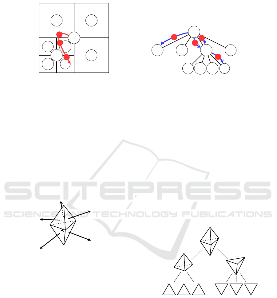
data saved for the original cell (see Figure 1). There

is a minimum size at which the cells will no longer

subdivide. The minimum size can be arbitrarily set

and should be adapted for the scene. A typical value

would be the smallest distance between any two light

sources in the scene.

When data is saved in a node, the full chain of par-

ent nodes are updated with the same data. This is to

make sure that when a lookup occurs for cells that are

further away from the user, there will at least be rel-

evant data saved, instead of some default value. This

situation can typically happen with animated objects.

For example, in Figure 1, when the user reaches the

third sample point in I, and then spawn an animated

object that travels into E. There is no data saved in E,

but there is recent data saved in A from when I got

updated that can be used as an approximation.

A natural expansion of this would be to use an

octree to store lighting information in three dimen-

sions. As our goal was to implement a simple and

performant method, we opted for a two-dimensional

data structure, which should cover the common case

of a user wearing an AR device and walking around a

scene with varying lighting.

3.2 Triangular Bipyramid

So far we have not mentioned how the directional in-

formation of the camera parameters is saved within

each node in the quadtree. We want our cell data

to cover incoming light from several directions, but

at the same time account for that there may only be

sampled data for a few of them. This depends on to

where the user is turning with the head-mounted cam-

era. Since the algorithm is meant to run on a head-

mounted device, and not rely on a high-performance

computer, the probe has to be able to be constructed

and read-back easily. For this we decided to use a

six-sided representation where the six sides are dis-

tributed around a triangular base. This allows us to

have each direction cover 120°. Each node saves six

sets of the camera parameters. Each set represents a

different direction and can be thought of as the surface

normals of a triangular bipyramid. Figure 2 visual-

izes these normals vectors. This distribution of nor-

mal vectors gives us three sample directions pointing

up, where would expect to get more direct sampling

GRAPP 2024 - 19th International Conference on Computer Graphics Theory and Applications

294

B C

D E

F G

H I

Spatial representation

B C D E

F G H I

Tree representation

Figure 1: Visualization of the quadtree. The quadtree is initialized around the user, with the origin in A. This becomes the

root of the quadtree and gets populated with available data. As the user traverses the scene (the red arrow), the camera will

sample new colour information and update the quadtree (blue arrows). Here the samples are noted as 1, 2, and 3. The ﬁrst

sample will force a subdivision of the quadtree and save its value to the corresponding cell—in this case B. For the subsequent

sample, 2, the user has moved and the value in D will be updated, since it is the ﬁrst value for this cell. For the last sample

there is already data in D, so a subdivision is forced, and a new value is saved in I. As values are saved in leaf nodes, the full

chain of parent nodes are also updated. So with the third sample, updating I, both A and D would also be updated and hold

the same value.

of the light sources (ceiling lights or sun), and three

samples directions pointing down, giving us informa-

tion about ambient lighting conditions. The triangular

base of the bipyramid could be exchanged for a geom-

etry with more sides, yielding more sample directions

and a more accurate lighting model, but at the cost of

higher complexity of the hierarchical structure.

Figure 2: The triangular bipyramid consists of two tetrahe-

dra that share one face. In our implementation we calcu-

lated our direction vectors from the normal vectors of the

faces. We used equilateral triangles to construct the trian-

gular bipyramid, this could however be changed to change

how much up or down the normals are pointing.

As the camera parameters are saved in the

quadtree, the viewing direction, calculated from the

user’s pose via the view matrix, is used to determined

which of the six faces of the triangular bipyramid the

data belongs to. This is done by projecting the view-

ing direction on all the normals and picking the nor-

mal that has the largest positive projection.

As the quadtree was picked and designed to han-

dle sparse samples from the camera, because it relies

on where the user has been in the scene to accurately

render objects, as must the triangular bipyramid be

able to provide data for directions that the user might

not have been looking in while sampling camera pa-

rameters from the scene. Using the same concept as

for the quadtree nodes, and reasoning that if we have

data for one of the directions, it can be reused as an

approximation until more accurate data is acquired.

We structure the triangular bipyramid’s faces in a tree

structure and make sure that when one node or face

is updated, the chain of parent nodes are updated as

well. This means that if a direction is not found, its

parent node, or parent of the parent, will always have

data (see Figure 3).

Figure 3: When retrieving values from the triangular bipyra-

mid, this tree structure is used to account for faces that are

potentially missing data. If a face is missing during data

lookup, the parent node is used instead, which is either the

top half or the bottom half of the bipyramid. If there is no

data in the parent, the latest saved data of any face is used,

which will be stored in the root node.

Spherical harmonics (SH) has been a popular

technique for constructing scene probes in prior work.

We did not use SH because sufﬁcient lighting in-

formation is rarely available to construct SH, and

the computational complexity would impact perfor-

Sparse Spatial Shading in Augmented Reality

295

mance. With a hierarchical probe, we can make sure

that we get some scene-relevant data when we sample

a sparsely populated probe.

3.3 Increasing Temporal Stability

To help with temporal stability of the saved data, and

avoid ﬂickering during colour correction, exponential

smoothing is used. When saving new sample data in

a node that already contains data, the new data will

be a weighted value between the new sample and the

old data. For a new data sample, x

, at time t, the data

value that is saved in a node, s

, can be calculated as

= αx

+ (1 − α)s

t−1

for t > 0 and 0 < α < 1, where s

t−1

is the old node

value and α is a weighting factor. This factor should

be tuned for the scene and the hardware as it depends

on if there are a lot of changing light conditions in the

scene or if the camera is reporting noisy values. We

found that using α = 0.5 worked well for our setup.

3.4 Shading Model

When an object is to be rendered, the lighting infor-

mation from the scene is collected from the quadtree

and sent to the pixel shader as six sets of camera pa-

rameters, corresponding to the six directions of the

triangular bipyramid. Once in the pixel shader, the

colours of the object are shaded to look like they are

affected by the surrounding real-world environment.

As mentioned in the beginning of Section 3, the

tracked camera parameters are:

• Lux estimation of scene

• Correlated colour temperature (CCT)

• Colour of the brightest pixels

The lux estimation and CCT are both readily avail-

able from our camera and are calculated from the ex-

posure and gain settings, and the auto white balanc-

ing algorithm respectively. The colour of the brightest

pixels can be calculated from the video stream.

3.4.1 Lux Estimation

We use the lux estimation to scale the brightness of

the rendered objects. As the lux values are not linear

in nature, we take the logarithm of the lux values to

get a linear relation between lux values and perceived

brightness (Microsoft, 2021).

Linearized light =

log

(lux value)

5.0

(1)

3.4.2 Transforming the CCT

To calculate how to transform the colour of the

rendered objects, the lighting information about the

scene is transformed into the CIE 1931 XYZ colour

space, before converting it to RGB for rendering.

Kang et al. (2002) offer an approximative numer-

ical approach of reconstructing CIE xyY coordinates

from a given black body temperature, T , in the range

1667K – 25000 K:

= a

+ b

+ c

+ d

, (2)

= a

+ b

+ c

+ d

, (3)

with the coefﬁcients given in Table 1. Note that the

coefﬁcients depend on the temperature interval.

The relationship between CIE xyY and CIE XYZ

is then as follows:

X =

, Y = Y, Z =

(1 − x − y)Y

. (4)

3.4.3 Colour of the Brightest Pixels

The colour of the brightest pixels are not calculated in

the camera’s internal algorithms, so it has to be done

manually. We do this by looping over all the pixels

in the image feed and checking for the highest valued

pixels. As the brightest pixels in a low-dynamic range

camera might very well saturate, we take the mean of

the pixels which have a colour channel value above

a certain threshold, but not saturated in any of the

colour channels. In our algorithm we used a threshold

of 235 (out of 255).

3.4.4 Shading Virtual Object

To render a virtual object so that it blends with the

real-world scene, we shift the white point of the vir-

tual object to that of the scene. The white point con-

version is done through a chromatic adaptation trans-

form and one of the more common ones is derived

from von Kries’ Koefﬁzientensatz (von Kries, 1905).

For an object lit by a light source with white point A,

the tristimulus colour values for the same object as if

lit by a light source with white point B can be calcu-

lated as:

, (5)

GRAPP 2024 - 19th International Conference on Computer Graphics Theory and Applications

296

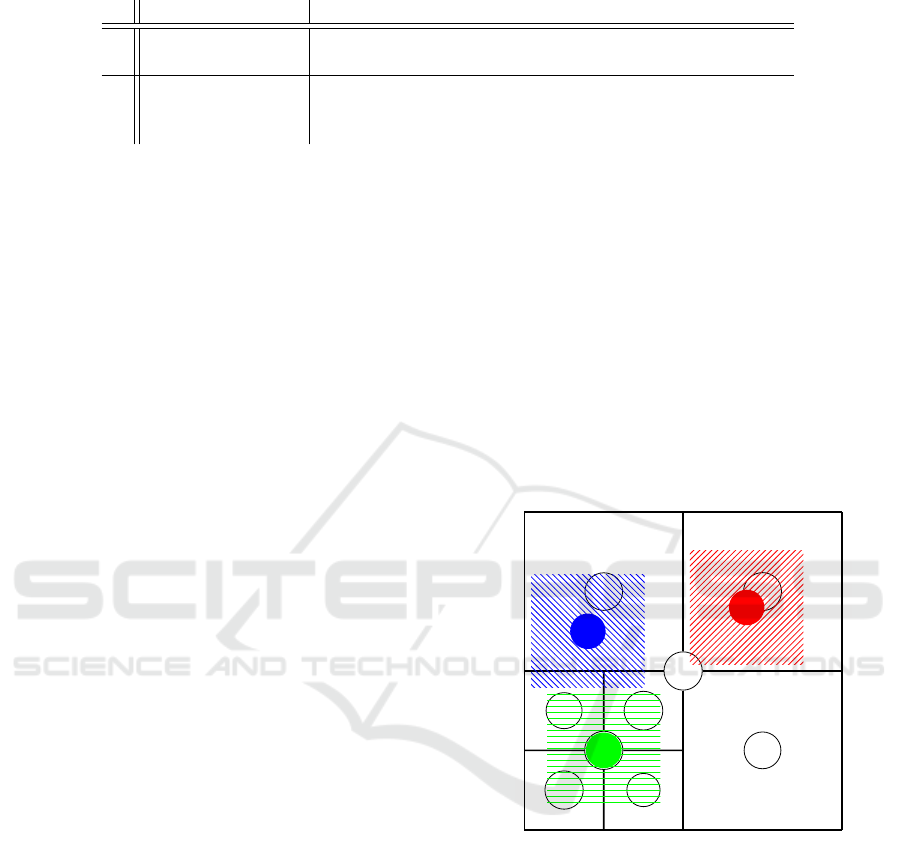
Table 1: Coefﬁcients for Equations (2) and (3).

T a b c d

1667K – 4000K -0.2661239 -0.2343589 0.8776956 0.179910

4000K – 25000 K -3.0258469 2.1070379 0.2226347 0.24039

1667K – 2222K -1.1063814 -1.34811020 2.18555832 -0.20219683

2222K – 4000K -0.9549476 -1.37418593 2.09137015 -0.16748867

4000K – 25000 K 3.0817580 -5.8733867 3.75112997 -0.37001483

where (R, G, B)

is the tristimulus value of the object

under light source A and (R, G, B)

is the same under

light source B. Subscript WP denotes the tristimulus

value at the white point for the different light sources.

3.4.5 Full Shading Algorithm

All the steps of the full shading algorithm are as fol-

lows:

1. Get the XYZ colour coordinate of the CCT using

Equations (2), (3) and (4)

2. Transform the brightest pixels mean RGB colour

value to XYZ colour space

3. Find midpoint between CCT and mean brightest

pixels in XYZ colour space

4. Transform the midpoint value to RGB colour

space

5. Transform lux estimation to a linearized light

level value using Equation (1)

6. Scale the RGB values with the linearized light

level value

7. Transform object colour with the estimated scene

RGB value using Equation (5)

8. Gamma correct ﬁnal colour into sRGB

By interpolating between the brightest pixel mean and

the CCT curve in XYZ space (point 3 above), the

colour from the CCT estimate can be extended to new

colours. The reason for using the CCT as a basis

is that it covers the most common and natural light

sources. Interpolating towards the brightest colour in

the scene allows for more “extreme” coloured light

sources to be compensated. Extreme in the sense

that the light sources are not well approximated by

a black-body radiator.

For point 7 above, the white point of the

HoloLens 2 is not known and for Equation (5) in our

implementation A

= (1, 1, 1) is used.

In the pixel shader, the normal vector of the frag-

ment being shaded is projected onto the six normals of

the triangular bipyramid and then the normalized con-

tribution of the positive projections are used to apply

the colour calculated from the camera parameters.

3.5 Increasing Spatial Stability

As the user traverses the scene, the colour correction

applied to the rendering has to change accordingly.

We want to use sample values from the quadtree that

is close to where the user is situated. To achieve

this, and without introducing ﬂickering artefacts as

the user passes from one node to the next one, we

sample a bigger region around the user’s position and

interpolate the ﬁnal colour correction parameters (see

Figure 4).

During construction of six sets, their values are

interpolated from all the quadtree cells that overlap

with the look-up area of the object.

B C

D E

F G

H I

Figure 4: This is how the weighting is done during a

quadtree lookup. In the ﬁgure, three objects are being ren-

dered (noted as 1, 2, and 3), and they perform lookups in

their immediate surrounding of the quadtree. How much

each node of the quadtree contributes to the ﬁnal colour

correction of a rendered object is determined by the over-

lapping areas of the objects look-up area and the area cov-

ered by a quadtree node. In this example, the look-up area

of object 1, shown in blue, covers B, F, and G. The con-

tributions are weighted according to the area of the overlap

and B will account for the majority the information, while F

and G will only contribute a small amount. Object 2, shown

in red, will only use colour correction data from C, whereas

object 3 will take equal amounts of F, G, H, and I.

Sparse Spatial Shading in Augmented Reality

297

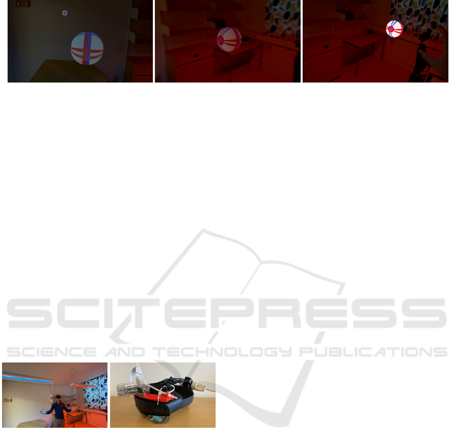
(a) Rendered ball under blue light. (b) Rendered ball under red light. (c) Unshaded ball.

Figure 5: (a) and (b) show a ball with red and blue stripes shaded by blue and red lights from the scene. In (c) the same ball

is rendered under the red light, but without any colour correction.

4 EVALUATION AND RESULTS

To test the algorithm, a scene with mixed-colour ceil-

ing lights was constructed. A room with ﬂuorescent

ceiling light was used, and we covered the lights with

differently coloured acrylic sheets. Figure 6 shows

a picture of the scene being used for testing. Also

presented in Figure 6 is the hardware we used to

evaluate the algorithm. Our implementation ran on

a HoloLens 2 from Microsoft, on top of which a

Raspberry Pi with a camera module was mounted.

The Raspberry Pi supplied the camera image param-

eters to the HoloLens 2 via a socket connection over

a wireless router. The reason for using an external

camera, as opposed to the camera that is part of the

HoloLens 2, was to gain more control over the image

parameters and at a lower level than the HoloLens 2

camera allowed.

(a) Scene. (b) Hardware.

Figure 6: (a) Scene with light sources in different colours.

(b) HoloLens 2 with Raspberry Pi and camera mounted on

top with the help of a 3-D printed bracket. Power supply for

the Raspberry Pi is supplied by an extension cable going to

the wall socket.

The mixed-reality video capture feature the

HoloLens 2 can be used to capture the video of the

internal HoloLens 2 camera with overlaid rendered

images. Figure 5 shows snapshots from the video

recorded using mixed-reality video capture in the test

scene. The full video can be found in the supplemen-

tal material of this paper. For the quadtree we set a

scene size of 20 × 20 metres and with a minimum cell

size of 0.625 × 0.625 metre. This is equal to 5 sub-

divisions, yielding a 32 × 32 uniform grid for a fully

sampled scene.

5 DISCUSSION

Our results show a promising way of colour correct-

ing rendered objects in AR applications. Figure 5

shows that using the colour correction, the balls are

more naturally part of the scene. In contrast, the un-

shaded ball looks like it is very obviously overlaid on

top of the background and not in the scene itself. All

this works even though the spatial data structure is

sparsely populated.

Our method utilizes only camera parameters and

sensory input that are readily available in AR devices

with built-in photo-grade cameras and motion track-

ing. For scenes with only common types of light

sources or natural daylight, the algorithm could be

simpliﬁed to only use the CCT data to do the colour

correction and no estimation of the brightest pixels

in the camera would be needed. The motivation to

also track the brightest pixels was that the CCT com-

pensation alone was very subtle because of the lim-

ited colour gamut of the holographic display in the

HoloLens 2.

5.1 Limitations and Future Work

The evaluation of our results have so far been limited,

and an extended assessment is needed, and potentially

a user study should be performed to complement the

results.

In the current implementation every object per-

forms one lookup in the quadtree as it is rendered.

For large objects spanning several quadtree cells, sev-

eral lookups should be performed to achieve an ac-

curate shading. Large objects would currently only

be shaded uniformly as per the cell where the object

deﬁnes its origin.

Different types of spatial data structures could be

tested, and especially the directional structure, the tri-

angular bipyramid, could be replaced with something

else, for instance spherical harmonics could be evalu-

ated as an alternative.

GRAPP 2024 - 19th International Conference on Computer Graphics Theory and Applications

298

Regarding the colour uniformity of the display,

optimally the colour of the display and its colour

gamut should be considered as well to recreate an

accurate colour. The result could then be evaluated

with sensors reading the display colour. The display

should then render an object with a real world coun-

terpart, also placed in the scene under the same light,

and the sensor readings could be compared to that of

the real object.

Finally, we had to use an external camera con-

nected to a Raspberry Pi to get the camera values we

needed. Preferably, this should be done with the cam-

eras already part of the AR device itself.

6 CONCLUSIONS

We have in this work presented a method for shading

objects in AR applications. Our approach is designed

with head-mounted AR devices in mind, both in terms

of how we expect our samples from the head-mounted

camera to be unstructured and sporadic, as well as

employing data structures that can perform well on

low performance devices.

ACKNOWLEDGEMENTS

This work was supported by the strategic research en-

vironment ELLIIT.

REFERENCES

Calian, D. A., Mitchell, K., Nowrouzezahrai, D., and Kautz,

J. (2013). The shading probe: Fast appearance acqui-

sition for mobile ar. In SIGGRAPH Asia 2013 Techni-

cal Briefs, SA ’13, New York, NY, USA. Association

for Computing Machinery.

Kang, B., Moon, O., Hong, C., Lee, H., Cho, B., and Kim,

Y.-s. (2002). Design of advanced color: Temperature

control system for HDTV applications. 41(6):865–

871.

Klein, G. and Murray, D. (2009). Parallel tracking and map-

ping on a camera phone. In Proc. Eigth IEEE and

ACM International Symposium on Mixed and Aug-

mented Reality (ISMAR’09), Orlando.

Knecht, M., Traxler, C., Purgathofer, W., and Wimmer, M.

(2011). Adaptive camera-based color mapping for

mixed-reality applications. In 2011 10th IEEE Inter-

national Symposium on Mixed and Augmented Real-

ity, ISMAR 2011, pages 165–168.

Microsoft (2021). Understanding and interpret-

ing lux values. https://docs.microsoft.com/en-

us/windows/win32/sensorsapi/understanding-and-

interpreting-lux-values. Accessed: 2022-06-23.

Nowrouzezahrai, D., Geiger, S., Mitchell, K., Sumner, R.,

Jarosz, W., and Gross, M. (2011). Light factorization

for mixed-frequency shadows in augmented reality. In

2011 10th IEEE International Symposium on Mixed

and Augmented Reality, pages 173–179.

Oskam, T., Hornung, A., Sumner, R. W., and Gross, M.

(2012). Fast and stable color balancing for images

and augmented reality. In Visualization Transmission

2012 Second International Conference on 3D Imag-

ing, Modeling, Processing, pages 49–56. ISSN: 1550-

6185.

Rohmer, K., B

uschel, W., Dachselt, R., and Grosch, T.

(2014). Interactive near-ﬁeld illumination for pho-

torealistic augmented reality on mobile devices. In

2014 IEEE International Symposium on Mixed and

Augmented Reality (ISMAR), pages 29–38.

Rohmer, K., Jendersie, J., and Grosch, T. (2017). Nat-

ural environment illumination: Coherent interactive

augmented reality for mobile and non-mobile devices.

IEEE Transactions on Visualization and Computer

Graphics, 23(11):2474–2484.

Sabbadin, M., Palma, G., Banterle, F., Boubekeur, T., and

Cignoni, P. (2019). High dynamic range point clouds

for real-time relighting. Computer Graphics Forum,

38(7):513–525.

Seo, S., Kang, D., and Park, S. (2018). Real-time adaptable

and coherent rendering for outdoor augmented real-

ity. EURASIP Journal on Image and Video Process-

ing, 2018(118).

von Kries, J. (1905). Die Gesichtsempﬁndungen, volume 3

of Handbuch der Physiologie des Menschen. Braun-

schweig, Vieweg und Sohn.

Sparse Spatial Shading in Augmented Reality

299