Convolutional Neural Networks and Image Patches for Lithological
Classification of Brazilian Pre-Salt Rocks
Mateus Roder
2
, Leandro Aparecido Passos
1
, Clayton Pereira
1
, Jo
˜
ao Paulo Papa
1
,
Altanir Flores de Mello Junior
3
, Marcelo Fagundes de Rezende
3
, Yaro Mois
´
es Parizek Silva
3
and Alexandre Vidal
2
1
Department of Computing, S
˜
ao Paulo State University (UNESP), Brazil
2
Institute of Geosciences, Campinas State University (UNICAMP), Brazil
3
Research Center, Leopoldo Am
´
erico Miguez de Mello Research, Development and Innovation Center (Cenpes), Brazil
Keywords:
Lithological Classification, Pre-Salt Rocks, Convolutional Neural Networks.
Abstract:
Lithological classification is a process employed to recognize and interpret distinct structures of rocks, provid-
ing essential information regarding their petrophysical, morphological, textural, and geological aspects. The
process is particularly interesting regarding carbonate sedimentary rocks in the context of petroleum basins
since such rocks can store large quantities of natural gas and oil. Thus, their features are intrinsically cor-
related with the production potential of an oil reservoir. This paper proposes an automatic pipeline for the
lithological classification of carbonate rocks into seven distinct classes, comparing nine state-of-the-art deep
learning architectures. As far as we know, this is the largest study in the field. Experiments were performed
over a private dataset obtained from a Brazilian petroleum company, showing that MobileNetV3large is the
more suitable approach for the undertaking.
1 INTRODUCTION
In recent years, a more profound petrographic com-
prehension of rock types within petroleum basins has
emerged as a crucial tool for enhancing data refine-
ment in engineering and geology. This understanding
aids in optimizing the efficient extraction of this sig-
nificant fossil fuel. Moreover, lithology identification
offers invaluable insights into the petrophysical char-
acteristics of oil and gas reservoirs, including porosity
and permeability. (Xu et al., 2021; Faria et al., 2022).
The analysis of rock and slide images from thin
section play a pivotal role in various geoscience ap-
plications. This analysis yields precise insights into
mineral composition and porosity, facilitates the iden-
tification of elements affecting fluid dynamics, en-
ables the estimation of reservoir quality, and enhanc-
ing lithological identification (Xu et al., 2022).
As the accurate classification of rock samples is
pivotal in this field, the academic community has
been diligently developing tools to streamline the au-
tomated classification of thin section microscopy im-
ages. These tools often integrate machine learning
and deep learning algorithms, harnessing the power
of computer vision for tasks such as rock thin section
classification (Polat et al., 2021; Xu et al., 2021; Faria
et al., 2022).
In this context, Ghiasi-Freez et al. (Ghiasi-
Freez et al., 2014) proposed an artificial neural net-
work (ANN) to classify carbonate rocks into grain-
stone, wackestone, mudstone, and packstone, while
Młynarczuk et al. (Młynarczuk et al., 2013) employed
traditional machine learning techniques to perform
classification over nine types of rocks. More recent
works used deep learning architectures for the task,
de Lima et al. (de Lima et al., 2019), for instance,
employed convolutional neural networks (CNNs) to
identify microfacies, while Nanjo et al. (Nanjo and
Tanaka, 2019) applied a similar procedure to identify
different lithologies in carbonate rocks. Further ap-
plications involving deep architectures for rock type
classification are addressed in (Cheng and Guo, 2017;
Faria et al., 2022; Xu et al., 2021).
This paper proposes a comparison of nine deep
architectures for the task of carbonate rocks lithol-
ogy classification into seven distinct classes, namely
648
Roder, M., Passos, L., Pereira, C., Papa, J., Mello Junior, A., Fagundes de Rezende, M., Silva, Y. and Vidal, A.
Convolutional Neural Networks and Image Patches for Lithological Classification of Brazilian Pre-Salt Rocks.
DOI: 10.5220/0012429100003660
Paper published under CC license (CC BY-NC-ND 4.0)
In Proceedings of the 19th International Joint Conference on Computer Vision, Imaging and Computer Graphics Theory and Applications (VISIGRAPP 2024) - Volume 3: VISAPP, pages
648-655
ISBN: 978-989-758-679-8; ISSN: 2184-4321
Proceedings Copyright © 2024 by SCITEPRESS – Science and Technology Publications, Lda.

Clay Spherulite, Spherulite, Grainstone, Dolomite,
Arborescent Stromatolite, Laminite, Rudstone. Ex-
periments were conducted over a private dataset of
petrographic thin section images of carbonate rocks
extracted over two oil wells by a Brazilian petroleum
company. The main contributions of this paper are
three-fold:
• to evaluate nine deep architectures in the context
of carbonate rocks classification;
• to scrutinize the quality of the oil reservoirs based
on the features observed on carbonate rocks that
compose the well basin;
• to foster the literature regarding oil reservoir qual-
ity assessment based on carbonate rocks’ classifi-
cation.
The remainder of this paper is organized as fol-
lows. Section 2 provides a theoretical background re-
garding CNNs and Pre-Salt Carbonate Rocks, while
Section 3 introduces the reader to the methods em-
ployed in this research. Further, Section 4 comprises
the results and discussions. Finally, Section 5 states
conclusions.
2 THEORETICAL BACKGROUND
AND RELATED WORKS
In this section, we present the main concepts of con-
volutional neural networks, and the lithographic rock
classification problem, as well as the main works re-
lated to this research.
2.1 Convolutional Neural Networks
Convolutional Neural Networks (LeCun et al., 1998)
have achieved exceptional popularity in the early
2010s, becoming fundamental for solving problems
related to image processing, such as image classifi-
cation (Sandler et al., 2018) and segmentation (Zoph
et al., 2020). As the name suggests, the main dif-
ference from the standard deep neural networks re-
lies on the neurons, convolutional-based ones, which
compose the basic blocks of CNNs, i.e., kernels re-
sponsible for performing convolution operations. By
applying a convolution kernel to the data, this opera-
tion generates a new set of matrices, which are used
as input data for the subsequent model layers. In sig-
nal processing, convolution is described as multiply-
ing two signals to generate a third (Oppenheim et al.,
2001).
CNNs were proposed with a base sequence of op-
erations i.e., convolutions, application of the activa-
tion function to their output, and, optionally, sampling
(pooling) (LeCun et al., 2010). As mentioned earlier,
the convolution represents the matrix multiplication
of the data window and a kernel. Subsequently, the
transformed data pass through an activation function,
whose options are numerous, such as sigmoid, hyper-
bolic tangent, and ReLu, for instance. In this step, the
linearity is broken, and naturally, the reduction of the
data dimension can occur.
Finally, the process can be followed by the out-
put dimension reduction via the pooling layer, usu-
ally choosing a window smaller than the kernel di-
mension. In this step, most applications use sam-
pling similar to a high-pass filter, letting only the
maximum values of each window pass (max-pooling).
The previously described steps and the learning pro-
cess on a CNN were discussed extensively by Ya-
mashita et al. (Yamashita et al., 2018). As the prob-
lems in computer vision become more challenger,
many convolutional architectures variants emerged in
the last decade, highlighting the residual-based CNN
(ResNet) (He et al., 2016) and the MobileNet (Sandler
et al., 2018).
2.2 Pre-Salt Carbonate Rock
Carbonate sedimentary rocks, formed by minerals
like dolomite and calcite, denote a particularly ap-
pealing type of sediment whose features are intrinsi-
cally correlated with the production potential of an oil
reservoir (Nanjo and Tanaka, 2019). Such a relation-
ship regards the sediment composition and structure,
which are especially attractive due to their capacity
to store large quantities of natural gas and oil inside
them (Worden et al., 2018).
The interpretation of carbonate rocks’ structure
may provide petrophysical, morphological, textural,
and geological aspects, like framework and diagenetic
composition, porous structure, and mineral distribu-
tion, among others, which contribute with valuable
information about the quality of the reservoirs (Gu
et al., 2018; Rabbani et al., 2017). However, inter-
preting such structures poses a complex problem due
to the deposition process, which entails internal di-
agenetic modifications in their structures (Burchette,
2012), thus demanding a detailed carbonate facies’
analysis for the identification of such aspects (Faria
et al., 2022).
In this context, carbonate lithology performs an
essential role, influencing the analysis of the reservoir
characteristics and geological modelling (Duan et al.,
2020), as well as providing imperative information re-
garding oil and gas petrographic features such as the
permeability and porosity of the reservoirs (Alzubaidi
et al., 2021).
Convolutional Neural Networks and Image Patches for Lithological Classification of Brazilian Pre-Salt Rocks
649

3 METHODOLOGY
In this section, we present an overall description of
the dataset and the experimental setup regarding the
proposed approach, with hyperparameters details.
3.1 Dataset
For this study, we used 62 private petrographic thin
section (“slide”) images of carbonate rocks, employ-
ing the automated mineralogical mapping (QEM-
SCAN) technique. Out of these images, 18 origi-
nated from samples extracted from oil well “A” (rang-
ing in depth from 5,026.05m to 5,091.65m), while
the remaining 44 was sourced from oil well “B” (with
depths spanning from 5,354.00m to 5,894.00m). In
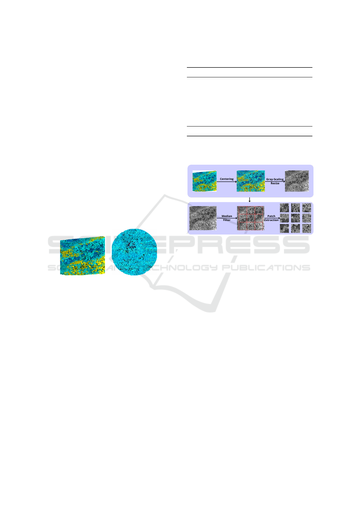
Figure 1, one can observe an illustrative sample slide.
The QEMSCAN method, an abbreviation for Quanti-
tative Evaluation of Minerals by Scanning Electron
Microscopy, is akin to a traditional scanning elec-
tron microscope coupled with EDS (Energy Disper-
sive Spectroscopy) detectors; However, it operates
in an automated manner, transforming chemical data
into mineralogy.
(a) (b)
Figure 1: Rock thin section from (a) oil well “A” and (b) oil
well “B”.
The dataset was curated by geological specialists,
in which the mineral’s composition and distribution
were deeply investigated, resulting in seven classes
for the sampled thin sections. Those classes are as
follows: Clay Spherulite (0), Spherulite (1), Grain-
stone (2), Dolomite (3), Arborescent Stromatolite (4),
Laminite (5), and Rudstone (6), with the number in
brackets representing the numerical equivalence of its
class. Table 1 shows the number of samples regarding
each class on the dataset, and its corresponding pro-
portion. Therefore, one can see the class imbalance
on the dataset, depicting a challenge.
Regarding the image properties, the thin sections
obtained with the QEMSCAN have not a standard res-
olution, i.e., some images have ≈ 2,500 × 2,000 pix-
els, while other ones have ≈ 2,000 × 2, 500 pixels, or
the region of interest is a small circumference inside
the overall image. These facts depict a significant dif-
ficulty, requiring some pre-processing steps before the
Table 1: Class proportion over the dataset.
Class #Samples Proportion
Clay Spherulite 9 15%
Spherulite 8 14%
Grainstone 17 29%
Dolomite 4 7%
Arborescent Stromatolite 11 19%
Laminite 4 7%
Rudstone 6 10%
Total 59 100%
CNNs receive the data. In such a manner, a manual
crop was employed to remove large blank regions, as
depicted in Figure 2, marked as the centering step.
Figure 2: Pre-processing pipeline for generating the rock
patches.
Following the pre-processing pipeline in Figure 2,
the thin sections are converted into grayscale. Ad-
ditionally, we apply the median filter with a kernel
size of 3 pixels on the neighborhood to smooth the
pixel intensity and reduce the noise introduced by pre-
vious conversions. The next step represents the di-
vision of each image into several patches with dif-
ferent patch sizes. Regarding such division, we em-
ployed three patch sizes: 250 × 250, 200 × 200, and
150 × 150, with a stride of 200, 150, and 100, respec-
tively. Moreover, it is important to highlight that such
sizes facilitate the resize operation to feed the images
to CNN models since they have specific input dimen-
sions (covered in the next subsection).
3.2 CNN Models
The study comprises the fine-tuning of different CNN
architectures regarding the problem of rock image
thin section classification. Additionally, it covers
comprehension of the patch size influence on the net-
working processing and accuracy. Four main archi-
tectures were selected to study the patch size effect
on their performance and to discover the architecture
variation more suitable to the problem. The CNNs
chosen were: ResNet (18, 34, 50, 101) (He et al.,
VISAPP 2024 - 19th International Conference on Computer Vision Theory and Applications
650

2016), DenseNet (121, 161) (Huang et al., 2017), Mo-
bileNet V3 (small and large) (Howard et al., 2019),
ShuffleNet V2 (Ma et al., 2018). It is important to
cite that all models employed in this study were pre-
trained on the ImageNet dataset (Deng et al., 2009),
which comprises more than 14 million samples, and
1,000 classes.
In short, the ResNet (He et al., 2016) is an ar-
chitecture known for its remarkable performance in
image classification and computer vision tasks. The
main innovation of ResNet is the use of residual
blocks, also called skip connections or shortcut con-
nections. These blocks allow the network to skip one
or more layers and pass information from one layer to
another, which helps mitigate the vanishing gradient
problem. Such a procedure enables us to train very
deep neural networks ranging from 18 to more than
100 layers, which was challenging before ResNet.
The DenseNet (Huang et al., 2017), or Densely
Connected Convolutional Network, is a ResNet vari-
ant introduced to address challenges associated with
training very deep networks for image classification
and other computer vision tasks. The distinctive fea-
ture of DenseNet is its dense connectivity pattern. In
traditional CNNs, each layer is connected only to the
previous layer and the input; however, the DenseNet
establishes direct connections between each layer and
all subsequent layers in a feedforward manner. This
dense connectivity promotes feature reuse and facil-
itates the flow of gradients throughout the network,
which enables the training of up to 121 or 161 layers.
On the other hand, the MobileNet V3 (Howard
et al., 2019) is a lightweight deep neural network ar-
chitecture designed for mobile and edge devices and
is an evolution of the original MobileNet V2 (San-
dler et al., 2018). It introduces the concept of in-
verted residuals with linear bottlenecks, representing
the use of lightweight depthwise separable convolu-
tions with a shortcut connection, similar to ResNets.
The width multiplier and resolution multiplier allow
users to customize the model size, which names the
model in small or large, according to the setup. It
has demonstrated competitive performance on various
benchmark datasets while being significantly smaller
in size compared to larger architectures designed for
cloud-based scenarios.
ShuffleNet V2 (Ma et al., 2018) is an extension
of the original ShuffleNet, and it is designed to pro-
vide efficient channel shuffling and further improve
the performance of deep neural networks while main-
taining computational efficiency. The main inno-
vation of ShuffleNet V2 concerns its channel shuf-
fling operations, which help in exchanging informa-
tion across channels, allowing for efficient use of fea-
ture maps. Its basic building block is the ShuffleNet
unit, which consists of pointwise group convolution,
channel shuffle, depthwise convolution, and another
pointwise group convolution. This unit allows for ef-
ficient information exchange across channels.
3.3 Experimental Setup
Considering the CNNs input dimension limitation of
224 × 224 pixels and three channels (RGB), we re-
sized the image patches, i.e., the 250, 200, and the
150, to this shape. Additionally, since the pre-trained
models require three channels, and the grayscale
patches have one channel, we replicated it to form the
correct input shape, i.e., 224×224×3. In such a man-
ner, each CNN model was trained independently for
10 times to alleviate the stochastic behavior of param-
eters initialization and update.
Regarding the model’s fine-tuning, we froze all
the convolution layers and fine-tuned the model’s fi-
nal fully-connected layer (FC), appending another FC
with shape 1,000 × 7. We fine-tuned the models’ FC
with Adam (Kingma and Ba, 2015) optimizer, con-
sidering a learning rate of 1× 10
−4
, and the appended
FC also with Adam and a learning rate of 1 × 10
−3
,
for 10 epochs, with the cross-entropy loss. The batch
size was 32 samples, and a Dropout layer with a prob-
ability of 10% of neurons being dropped on the FC
layer from the model was employed. Such hyper-
parameters were empirically defined using the vali-
dation set (forward covered).
Additionally, one can define the data split em-
ployed in the experimental setup. This step stands for
a hold-out split with 85% of data to train, and 15%
to test, being 15% of the train set employed as the
validation set. Since the dataset is highly imbalanced
(Table 1), we opted to stratify the hold-out procedure
by the class, keeping the class proportion on the par-
titions (train, validation, and test). Furthermore, it is
meaningful to highlight that, by changing the patch
size, the amount of data available to the partitions
varies since we fixed the proportions instead of the
number of samples, which can generate more patches
when the patch size is reduced, for instance.
We employed four classical evaluation measures,
Precision, Recall, F1-score, and Accuracy, to evalu-
ate the models’ performance. Such measures depict a
standard evaluation approach for classification prob-
lems. Finally, to run the defined combinations of ex-
periments, we utilized an Intel Xeon with 32 cores,
128Gb of RAM, and a GTX TITAN X GPU with
12Gb of memory. Unfortunately, even though this
GPU enables us to run different models, more com-
plex ones or more samples on the batch were not pos-
Convolutional Neural Networks and Image Patches for Lithological Classification of Brazilian Pre-Salt Rocks
651

Table 2: Performance evaluation regarding the patches with
size 250.
Precision Recall F1 Accuracy
ResNet18 mean 0.5811 0.5673 0.5651 0.5673
std 0.0196 0.0245 0.0244 0.0245
ResNet34 mean 0.5912 0.5820 0.5785 0.5820
std 0.0304 0.0303 0.0293 0.0303
ResNet50 mean 0.6165 0.6034 0.5965 0.6034
std 0.0164 0.0176 0.0180 0.0176
ResNet101 mean 0.6410 0.6212 0.6160 0.6212
std 0.0281 0.0283 0.0286 0.0283
DenseNet121 mean 0.6447 0.6320 0.6263 0.6320
std 0.0214 0.0250 0.0254 0.0250
DenseNet161 mean 0.6658 0.6591 0.6561 0.6591
std 0.0133 0.0131 0.0144 0.0131
MobileNetV3small mean 0.6337 0.6185 0.6167 0.6185
std 0.0237 0.0108 0.0114 0.0108
MobileNetV3large mean 0.6974 0.6889 0.6869 0.6889
std 0.0182 0.0192 0.0205 0.0192
ShuffleNetV2 mean 0.6429 0.6327 0.6285 0.6327
std 0.0123 0.0128 0.0148 0.0128
sible due to the GPU memory consumption.
4 EXPERIMENTAL RESULTS
Regarding the experimental results, Tables 2, 3, and 4
present the mean and standard deviation for the test
set partition of the four evaluated metrics obtained
from ten independent repetitions, considering the
three patch sizes selected over all CNN models. Ad-
ditionally, best results are marked in bold.
From Table 2, one can observe the performance
improvement over the precision, recall, F1-score, and
accuracy for the ResNet models, which represents
that, by increasing the number of residual blocks, the
model learns more about the data and generalizes bet-
ter. Such scalability stands for almost 2% in accu-
racy, starting with ResNet18 with 0.5673 to 0.5820
on ResNet34, for instance. Analyzing the DenseNet,
we observed the same behavior from DenseNet121 to
DenseNet161, in which all measures were improved
with more dense blocks being employed, i.e., 121
versus 161. However, the performance improvement
over the previous models was not as accentuated as
the improvement from the MobileNet V3 small to the
large, with the larger model achieving a mean accu-
racy of 0.6889, an impressive result over all models,
even the ShuffleNet V2 (0.6327).
Regarding Table 3, one can perceive the same be-
havior previously observed, i.e., as the model com-
plexity increases, the performance measures increase
within the same model family. However, one can
see the ResNet101 surpassing both DenseNets in pre-
cision, recall, F1-score, and accuracy, which indi-
cates that a “simpler” model can benefit more than
“complex” models when more data is available, since
reducing the patch size the number of samples in-
Table 3: Performance evaluation regarding the patches with
size 200.
Precision Recall F1 Accuracy
ResNet18 mean 0.6465 0.6337 0.6296 0.6337
std 0.0208 0.0173 0.0178 0.0173
ResNet34 mean 0.6573 0.6420 0.6384 0.6420
std 0.0260 0.0278 0.0294 0.0278
ResNet50 mean 0.6921 0.6658 0.6621 0.6658
std 0.0178 0.0287 0.0317 0.0287
ResNet101 mean 0.7115 0.6963 0.6948 0.6963
std 0.0161 0.0203 0.0193 0.0203
DenseNet121 mean 0.6760 0.6599 0.6577 0.6599
std 0.0234 0.0189 0.0195 0.0189
DenseNet161 mean 0.6868 0.6777 0.6736 0.6777
std 0.0147 0.0133 0.014 0.0133
MobileNetV3small mean 0.6521 0.6460 0.6429 0.6460
std 0.0111 0.0146 0.0142 0.0146
MobileNetV3large mean 0.7194 0.7125 0.7105 0.7125
std 0.0174 0.0170 0.0179 0.0170
ShuffleNetV2 mean 0.6496 0.6401 0.6391 0.6401
std 0.0209 0.0219 0.0219 0.0219
Table 4: Performance evaluation regarding the patches with
size 150.
Precision Recall F1 Accuracy
ResNet18 mean 0.6575 0.6462 0.6442 0.6462
std 0.0096 0.0147 0.0134 0.0147
ResNet34 mean 0.6465 0.6372 0.6355 0.6372
std 0.0163 0.0177 0.0197 0.0177
ResNet50 mean 0.6927 0.6752 0.6722 0.6752
std 0.0149 0.0168 0.0166 0.0168
ResNet101 mean 0.7166 0.7081 0.7052 0.7081
std 0.0140 0.0157 0.0165 0.0157
DenseNet121 mean 0.6762 0.6643 0.6599 0.6643
std 0.0136 0.0169 0.0173 0.0169
DenseNet161 mean 0.6993 0.6921 0.6892 0.6921
std 0.0142 0.0129 0.0136 0.0129
MobileNetV3small mean 0.6649 0.6578 0.6564 0.6578
std 0.0124 0.0101 0.0100 0.0101
MobileNetV3large mean 0.7282 0.7237 0.7222 0.7237
std 0.0085 0.0091 0.0084 0.0091
ShuffleNetV2 mean 0.6263 0.6159 0.6130 0.6159
std 0.0088 0.0098 0.0115 0.0098
creases. Moreover, as expected, the MobileNet V3
large achieved better performance overall measures
and other models, while the ResNet101 ranked in sec-
ond place.
Regarding Table 4, the behavior observed in Ta-
bles 3 and 2 slightly changed, i.e., the ResNet34
did not improve its performance as expected and ob-
served on patches 250 and 200. However, once more,
the ResNet101 surpasses both DenseNets in preci-
sion, recall, F1-score, and accuracy, with all measures
greater than 0.70. Once again, the MobileNet V3
large achieved better performance over all measures
(greater than 0.72) and models, while the ResNet101
also ranked in second place. Finally, the ShuffleNet
V2 achieved the worst performance in all measures,
which is interesting since the model was not the worst
on previous patch sizes.
In summary, one can elucidate some key findings.
Firstly, the residual models achieved good perfor-
mance in all measures, highlighting the ResNet101,
which represents a good alternative for the pre-salt
VISAPP 2024 - 19th International Conference on Computer Vision Theory and Applications
652

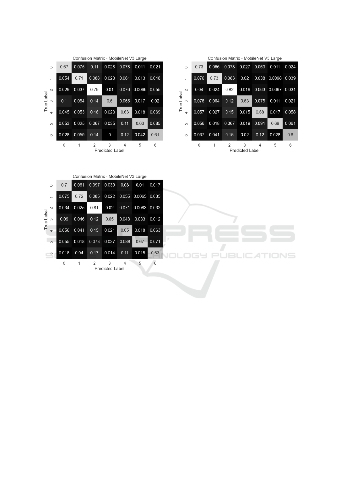
Figure 3: Confusion matrix for MobileNet V3 Large and
patch size of 250.
Figure 4: Confusion matrix for MobileNet V3 Large and
patch size of 200.
rock classification problem, especially if more data
is available to fine-tune. The second finding is that
MobileNet V3 large is more suitable to our prob-
lem, even with low data volume, since its results sur-
passed all models for the three patch sizes employed.
Moreover, a patch size of 150 seems to be a good al-
ternative, however, mainly when more data is avail-
able. As complementary results, the confusion ma-
trices averaged over the 10 repetitions, in percentage,
for the best model overall (MobileNet V3 large) are
presented in Figures 3, 4, and 5.
Finally, comparing Figures 3, 4, and 5, one can see
the performance improvement on the main diagonal,
from the 250 to 150 patch sizes. First, from Figure 3,
the greater error percentage classification stands for
predicting as class 2 the patches of class 4, i.e., 16%
of the test samples. Such an observation represents
a possible bias since class 2 has more data on the
Figure 5: Confusion matrix for MobileNet V3 Large and
patch size of 150.
dataset. Regarding Figure 4, the same behavior oc-
curred, i.e., more samples have been classified incor-
rectly as class 2 (column 2). Additionally, the main
diagonal increased its values. Lastly, Figure 5 gath-
ers the better result, with a substantial increase on the
main diagonal, and a reduction in samples incorrectly
classified as class 2 (column 2).
5 CONCLUSIONS
In this paper, we addressed the problem of pre-salt
rock lithology classification with convolutional neural
networks. In such a manner, the study objective was
to understand the learning and generalization capa-
bility of state-of-the-art pre-trained models employed
in a fine-tuning phase with low data availability and
high-class imbalance. Additionally, we extended our
investigation on the patch size used to crop the origi-
nal image thin section.
We employed a total of nine models, from
ResNets to MobileNets, trained on three different
patch sizes, 250, 200, and 150 pixels crop. The first
patch size leads us to deep models with all perfor-
mance measures greater than 0.56 percentage mean,
highlighting the MobileNet V3 large, with a mean
greater than 0.68, representing a good starting point,
since the dataset has only 59 thin sections.
Regarding the second and third patch sizes (200
and 150), we observed patterns in the models’ be-
havior, i.e., with more data available to train, the per-
formance increases for most of the employed models,
with the better one being the MobileNet V3 large so
far. Additionally, even with a small crop, 150 pix-
els, the resizing operation does not negatively inter-
fere. Regarding the best MobileNet, its superior per-
Convolutional Neural Networks and Image Patches for Lithological Classification of Brazilian Pre-Salt Rocks
653

formance indicates the model is a good candidate to
be deployed as we have more data collected to im-
prove the training.
Even with the promising results using image
patches to feed the architectures, it represents a chal-
lenge if we want to modify the patch size on a sub-
stantial scale, such as 500 or 50 pixels since the pre-
trained architectures have fixed input sizes. We expect
to explore this challenge by modifying the first layer
and resizing its output to match the original config-
uration, considering more data to train the required
lower-level layers.
Considering future works, we aim to deeply inves-
tigate modifications to the MobileNet architecture to
improve our results, and aggregate multimodal data.
Additionally, we expect to collect more data to train
models from scratch and compare it with its fine-
tuned version.
ACKNOWLEDGEMENTS
The authors are grateful to Petrobras-CENPES,
Brazil, for providing the oil well images and grant
#5472. Also, we are grateful to Fundac¸
˜
ao de Amparo
`
a Pesquisa do Estado de S
˜
ao Paulo (FAPESP), Brazil
grants #2023/10823 − 6, for their financial support.
REFERENCES
Alzubaidi, F., Mostaghimi, P., Swietojanski, P., Clark, S. R.,
and Armstrong, R. T. (2021). Automated lithology
classification from drill core images using convolu-
tional neural networks. Journal of Petroleum Science
and Engineering, 197:107933.
Burchette, T. P. (2012). Carbonate rocks and petroleum
reservoirs: a geological perspective from the indus-
try. Geological Society, London, Special Publications,
370(1):17–37.
Cheng, G. and Guo, W. (2017). Rock images classification
by using deep convolution neural network. In Jour-
nal of Physics: Conference Series, volume 887, page
012089. IOP Publishing.
de Lima, R. P., Bonar, A., Coronado, D. D., Marfurt, K.,
and Nicholson, C. (2019). Deep convolutional neural
networks as a geological image classification tool. The
Sedimentary Record, 17(2):4–9.
Deng, J., Dong, W., Socher, R., Li, L.-J., Li, K., and Fei-
Fei, L. (2009). Imagenet: A large-scale hierarchical
image database. In 2009 IEEE Conference on Com-
puter Vision and Pattern Recognition, pages 248–255.
Duan, Y., Xie, J., Li, B., Wang, M., Zhang, T., and Zhou, Y.
(2020). Lithology identification and reservoir char-
acteristics of the mixed siliciclastic-carbonate rocks
of the lower third member of the shahejie formation
in the south of the laizhouwan sag, bohai bay basin,
china. Carbonates and Evaporites, 35:1–19.
Faria, E., Coelho, J. M., Matos, T. F., Santos, B. C., Tre-
vizan, W. A., Gonzalez, J., Bom, C. R., de Albu-
querque, M. P., and de Albuquerque, M. P. (2022).
Lithology identification in carbonate thin section im-
ages of the brazilian pre-salt reservoirs by the com-
putational vision and deep learning. Computational
Geosciences, 26(6):1537–1547.
Ghiasi-Freez, J., Honarmand-Fard, S., and Ziaii, M. (2014).
The automated dunham classification of carbonate
rocks through image processing and an intelligent
model. Petroleum science and technology, 32(1):100–
107.
Gu, Y., Bao, Z., and Rui, Z. (2018). Prediction of shell
content from thin sections using hybrid image process
techniques. Journal of Petroleum Science and Engi-
neering, 163:45–57.
He, K., Zhang, X., Ren, S., and Sun, J. (2016). Deep resid-
ual learning for image recognition. In Proceedings of
the IEEE conference on computer vision and pattern
recognition, pages 770–778.
Howard, A., Sandler, M., Chu, G., Chen, L.-C., Chen, B.,
Tan, M., Wang, W., Zhu, Y., Pang, R., Vasudevan, V.,
et al. (2019). Searching for mobilenetv3. In Pro-
ceedings of the IEEE/CVF international conference
on computer vision, pages 1314–1324.
Huang, G., Liu, Z., Van Der Maaten, L., and Weinberger,
K. Q. (2017). Densely connected convolutional net-
works. In Proceedings of the IEEE conference on
computer vision and pattern recognition, pages 4700–
4708.
Kingma, D. P. and Ba, J. (2015). Adam: A method for
stochastic optimization. In 3rd International Confer-
ence on Learning Representations, ICLR.
LeCun, Y., Bottou, L., Bengio, Y., Haffner, P., et al. (1998).
Gradient-based learning applied to document recogni-
tion. Proceedings of the IEEE, 86(11):2278–2324.
LeCun, Y., Kavukcuoglu, K., and Farabet, C. (2010). Con-
volutional networks and applications in vision. In Pro-
ceedings of 2010 IEEE International Symposium on
Circuits and Systems, pages 253–256.
Ma, N., Zhang, X., Zheng, H.-T., and Sun, J. (2018). Shuf-
flenet v2: Practical guidelines for efficient cnn archi-
tecture design. In Proceedings of the European Con-
ference on Computer Vision (ECCV).
Młynarczuk, M., G
´
orszczyk, A., and
´
Slipek, B. (2013).
The application of pattern recognition in the automatic
classification of microscopic rock images. Computers
& Geosciences, 60:126–133.
Nanjo, T. and Tanaka, S. (2019). Carbonate lithology iden-
tification with machine learning. In Abu Dhabi Inter-
national Petroleum Exhibition and Conference, page
D021S060R001. SPE.
Oppenheim, A. V., Buck, J. R., and Schafer, R. W. (2001).
Discrete-time signal processing. Vol. 2. Upper Saddle
River, NJ: Prentice Hall.
Polat,
¨
O., Polat, A., and Ekici, T. (2021). Automatic clas-
sification of volcanic rocks from thin section images
VISAPP 2024 - 19th International Conference on Computer Vision Theory and Applications
654

using transfer learning networks. Neural Computing
and Applications, 33(18):11531–11540.
Rabbani, A., Assadi, A., Kharrat, R., Dashti, N., and Ay-
atollahi, S. (2017). Estimation of carbonates perme-
ability using pore network parameters extracted from
thin section images and comparison with experimental
data. Journal of Natural Gas Science and Engineer-
ing, 42:85–98.
Sandler, M., Howard, A., Zhu, M., Zhmoginov, A., and
Chen, L.-C. (2018). Mobilenetv2: Inverted residu-
als and linear bottlenecks. In Proceedings of the IEEE
conference on computer vision and pattern recogni-
tion, pages 4510–4520.
Worden, R., Armitage, P., Butcher, A., Churchill, J., Csoma,
A., Hollis, C., Lander, R., and Omma, J. (2018).
Petroleum reservoir quality prediction: overview and
contrasting approaches from sandstone and carbonate
communities. Geological Society, London, Special
Publications, 435(1):1–31.
Xu, Z., Ma, W., Lin, P., and Hua, Y. (2022). Deep learning
of rock microscopic images for intelligent lithology
identification: Neural network comparison and selec-
tion. Journal of Rock Mechanics and Geotechnical
Engineering, 14(4):1140–1152.
Xu, Z., Ma, W., Lin, P., Shi, H., Pan, D., and Liu, T.
(2021). Deep learning of rock images for intelligent
lithology identification. Computers & Geosciences,
154:104799.
Yamashita, R., Nishio, M., Do, R. K. G., and Togashi, K.
(2018). Convolutional neural networks: an overview
and application in radiology. Insights into imaging,
9(4):611–629.
Zoph, B., Ghiasi, G., Lin, T.-Y., Cui, Y., Liu, H., Cubuk,
E. D., and Le, Q. V. (2020). Rethinking pre-training
and self-training. arXiv preprint arXiv:2006.06882.
Convolutional Neural Networks and Image Patches for Lithological Classification of Brazilian Pre-Salt Rocks
655