Optimization of Active Region of Quantum Cascade Laser (QCL) by

Coupled Calculation of Genetic Algorithm and QCL Simulator

Shigeyuki Takagi

, Tsutomu Kakuno

, Rei Hashimoto

, Kei Kaneko

and Shinji Saito

Department of Electrical and Electronics Engineering, School of Engineering, Tokyo University of Technology,

1404-1 Katakura, Hachioji, Tokyo, Japan

Corporate Manufacturing Engineering Center, Toshiba Corporation, 33 Shinisogo, Isogo, Yokohama, Kanagawa, Japan

Keywords: Quantum Cascade Lasers, QCLs, Active Region, non-Equilibrium Green’s Function, Genetic Algorithm, GA,

Optimization, Gain, Wavelength, Injector Barrier, Well.

Abstract: We applied a coupled calculation of genetic algorithm and a quantum cascade laser (QCL) simulator

(nextnano.QCL) to calculate the gain that excites laser light in the active region of the QCL. The film

thicknesses of the nine layers constituting the active region were changed simultaneously, and the film

structure with the maximum gain was determined from 1000 type of film structures. The QCL simulator

incorporating a non-equilibrium Green's function was used to calculate the gain of the QCL, and the validity

of the simulation was evaluated using the active region structure reported in the previous paper. In the coupled

calculation of the QCL simulator and genetic algorithms, we used gain as an objective function and methods

of crossing, natural selection, and mutation simulating the evolutionary process of living organisms to

optimize the thickness of nine films. As a result of the optimization calculation, the optimized structure had

gain (78.44 cm

–1

) higher than that (50.01 cm

–1

) in a structure reported in a previous paper.

1 INTRODUCTION

Quantum cascade lasers (QCLs) are n-type

semiconductor lasers in which two types of

semiconductor film are alternately stacked, and the

laser light in the infrared region can be obtained (Faist

et al., 1994). Since the wavelengths of QCLs are in

the infrared region, they are expected to be applied to

trace gas analysis and remote gas detection (Faist et

al., 2016). It is necessary to develop a laser with a

wavelength suitable for measurement. With such

trace substance detection and gas detection from a

distance, a higher sensitivity is expected by

increasing the output. Since the amount of laser

absorption is measured in the detection of trace

substances, it is necessary to propagate along a large

optical path length. To develop such high-power

lasers, it is effective to utilize a simulator that can

predict the oscillation wavelength and gain.

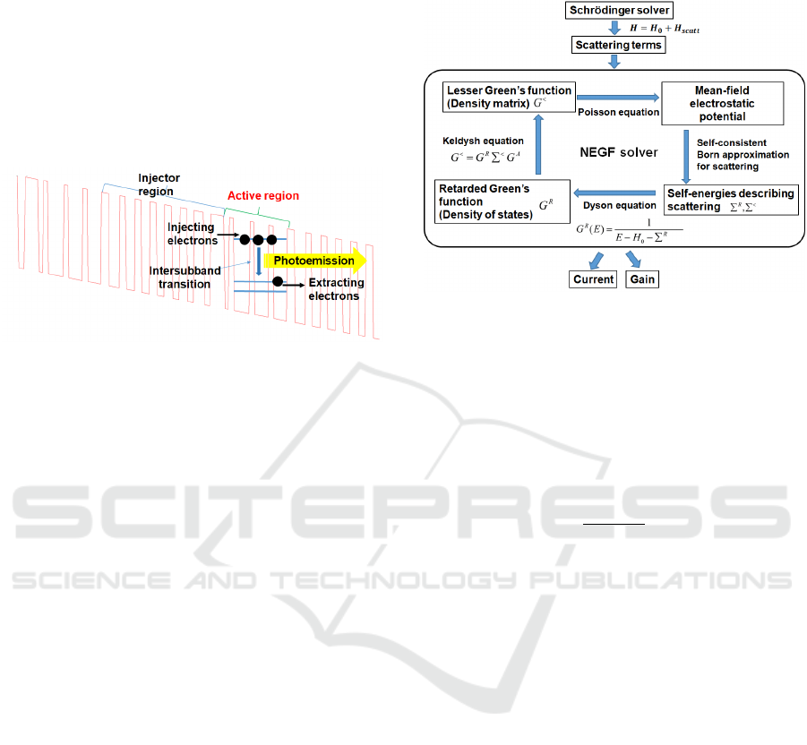
Figure 1 shows the band structure of a QCL. It has

an injector region that transports electrons and an

active region consisting of several sets of barrier and

https://orcid.org/0009-0009-6444-8748

https://orcid.org/0000-0002-1829-6482

well layers to excite laser light. Laser light is emitted

when electrons transition from an upper level to a

lower level in a quantum well formed in well layers.

In the current simulators, the Schrödinger equation is

solved to calculate the wave function, and the rate

equation solution method is used at the level, where

the electrons undergo transition. The amount of light

emitted is calculated semiclassically from the

lifetimes of the upper and lower levels, and the

transition probabilities between the upper and lower

levels (Lu et al., 2006). Recently, a calculation

method using the non-equilibrium Green's function

has been proposed (Grange, 2015). In the simulator,

the distribution of electron density and the transition

of electrons from the upper level to the lower level

can be calculated quantumly.

To increase the output of a QCL, it is necessary to

increase the intensity of the laser light excited in the

active region. An effective method is to use a QCL

simulator to optimize the thicknesses of the barrier

and well layers in the active region by increasing the

laser gain. However, the active region of a typical

Takagi, S., Kakuno, T., Hashimoto, R., Kaneko, K. and Saito, S.

Optimization of Active Region of Quantum Cascade Laser (QCL) by Coupled Calculation of Genetic Algorithm and QCL Simulator.

DOI: 10.5220/0012428200003651

Paper published under CC license (CC BY-NC-ND 4.0)

In Proceedings of the 12th International Conference on Photonics, Optics and Laser Technology (PHOTOPTICS 2024), pages 72-77

ISBN: 978-989-758-686-6; ISSN: 2184-4364

QCL is composed of four barrier layers and four well

layers. For this reason, the main method of

optimization thus far has been to fix some film

thicknesses and sequentially optimize the film

thickness. Otherwise, optimization was performed

under certain constraints, such as reducing the

thickness of all barrier layers by a certain percentage

(Tanimura et al., 2022). There are few reports on

methods for simultaneously optimizing all the layers

in the active region.

Figure 1: Band structure of QCL. (a) Injector region that

transports electrons and (b) active region that excites laser

light (Tanimura et al., 2022).

In this study, we developed an automatic

calculation method that combines a non-equilibrium

Green's function and a genetic algorithm (GA), and

applied the method to optimizing the film

thicknesses in the active region. Changing the

thicknesses of five types of barrier layer and four

types of well layers as parameters, we calculated the

gain and wavelength of 1000 types of the film

structures. As a result, a structure with optimized

film thickness was obtained with a gain (28.43 cm

–

) higher than that (50.01 cm

–

) in the QCL structure

reported in the paper. We also fabricated a prototype

QCL device, performed electro-luminescence (EL)

measurements, and verified the validity of the

optimized results.

2 QCL SIMULATOR

2.1 QCL Simulator Incorporating

non-Equilibrium Green's Function

We used nextnano.QCL (nextnano GmbH) as the

QCL simulator in this study (Grange, 2015). Figure 2

shows the calculation flow in the simulator. In the

Schrödinger equation, assuming that the unperturbed

Hamiltonian is H

and the electron scattering is the

perturbed Hamiltonian H

scatt

, the Hamiltonian H in

the Schrödinger as

H=



+



(1)

Using this Hamiltonian, we solved the Schrödinger

equation and calculated the electron orbit.

Figure 2: QCL simulator incorporating non-equilibrium

Green's function (Tanimura et al., 2022).

Next, we solved Poisson's equation to find the

mean-field electrostatics potential and calculated the

self-energy Σ

of delay and the self-energy Σ

Lesser, which describes electron scattering. The

Density of States (DOS) was obtained from the

delayed Green's function G

using the Dyson

equation as follows;











∑



.

(2)

Using the Keldysh equation shown in equation (3),

we calculated the electron density matrix from the

Lesser Green's function G





=











(3)

where G is the advanced Green's function. Current

and gain were calculated based on the basis of the

obtained electron density matrix.

From the calculation flow in Fig. 2, the relationship

between emitted energy (wavelength) and gain was

calculated. By using a non-equilibrium Green's

function, we effect such as the crystal lattice and

electron scattering. This is considered a major

advantage over conventional semiclassical

calculation methods.

2.2 Evaluation of Simulation Model

To examine the validity of this simulator, we inputted

the film structure and composition reported previously

into the QCL simulator (Evans et al., 2007). The film

structure was modeled using two sets of injector and

active regions. We assumed that the maximum gain

obtained in the simulation was the laser oscillation

wavelength and compared it with the oscillation

Optimization of Active Region of Quantum Cascade Laser (QCL) by Coupled Calculation of Genetic Algorithm and QCL Simulator

wavelength in the previous paper (Takagi et al., 2021).

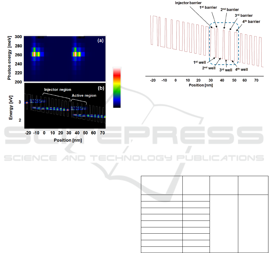
Figure 3 shows the calculation results. Figure 3(a)

shows the gain intensity and Fig. 3(b) shows the DOS

distribution. The horizontal axes in both (a) and (b)

indicate the position of the QCL film. As shown in

Fig. 3(a), a high gain was observed at the position

corresponding to the active region. The photon

energy of this gain was 260 meV, which corresponds

to a light wavelength of 4.77 nm. The oscillation

wavelength obtained by Evans et al. in their

experiment was 4.71 nm (Evans et al., 2007), which

is in good agreement with that in our simulation.

Figure 3: Calculation results of QCL simulator. (a) Gain

intensity and (b) DOS.

In Fig. 3(b), there are two stages of electron

distribution in the active region, and the upper and

lower electron distribution regions correspond to the

upper and lower levels of laser oscillation,

respectively. In addition, electrons with almost the

same energy level are distributed in the injector

region, indicating that electrons propagated through

the injector region. Nextnano.QCL was able to

accurately model electron propagation and laser light

emission. As a result, we were able to obtain the same

calculation results for the oscillation wavelength as

the experimental results.

3 COUPLED CALCULATION OF

GENETIC ALGORITHMS AND

QCL SIMULATOR

3.1 Optimization of Parameters

We optimized the structure of the active region that

excites the laser beam shown in Fig. 4. In the active

region, the barrier layer was formed with In

0.363

AlAs,

and the well layer was formed with In

0.669

GaA. The

thicknesses of the nine layers were optimized from

the injector barrier to the fourth barrier layer. The

reference structure of the active region was set to the

same structure of the QCL reported by Evans et al.

(Evans et al., 2007).

Figure 4: Optimizing film thicknesses in active region.

Table 1 shows the ranges of film thicknesses in

the active region. The thickness of each film was

varied within a range of ±1.0 nm from the reference

film thickness. Moreover, for films prepared by

Molecular beam epitaxy (MBE), their thicknesses are

less than 1.0 nm are difficult to control. Therefore, the

minimum film thickness was set to 1.0 nm.

Table 1: Ranges of film thicknesses of barrier and well

layers.

Barrier/well Film

material

[nm]

Thickness

range

[nm]

Minimum

thickness

[nm]

Injector barrier 3.8

± 1.0 ≧1.0

well 1.2

barrier 1.3

well 4.3

barrier 1.3

well 3.8

barrier 1.4

well 3.6

barrier 2.2

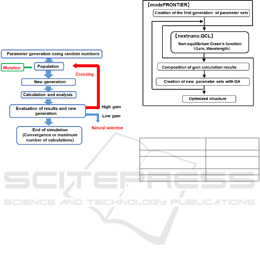
3.2 GA and Optimization Method

To optimize the active region, we developed a

calculation method that combines nextnano.QCL and

GA. GA is an evolutionary computational method for

solving optimization problems. It is one of the search

methods that can rapidly find the optimal solution, as

shown in Fig. 5 (Holland, 1975); (Holland,1992).

This algorithm reflects the evolutionary process of

PHOTOPTICS 2024 - 12th International Conference on Photonics, Optics and Laser Technology

living organisms in its optimization process and

consists of three distinctive methods: crossing,

natural selection, and mutation. Crossing and natural

selection can efficiently generate better parameter

combinations. Furthermore, mutation enables the

finding of the optimal solution for parameters that are

far from the initial conditions (Takagi et al., 2023).

Figure 5: Optimization flow using GA.

The optimization software modeFRONTIER

incorporating NSGA-II was used for GA calculations.

NSGA-II is a GAs proposed by Debi et al. (Debi et

al., 2022). It has excellent convergence and

computational stability. Figure 6 shows the flow of

the coupled calculation of modeFRONTIER and

nextnano.QCL. Table 2 shows the calculation method

and setting parameters. In this calculation, the gain

and wavelength were extracted from the results of

calculation using nextnano.QCL.

In the optimization, the parameter sets that

maximize gains as the objective function were

calculated. Furthermore, under the conditions where

the wavelength was not in the range from 4.0 µm to

5.0 µm, we judged the parameter sets to be

inappropriate. In the calculation using the GA, 10

parameter sets were calculated simultaneously as the

same generation, and 10 new parameter sets in the

next generation were created using the gain and

wavelength as evaluation indicators. These

calculation processes were repeated 100 times, and

1000 types of the parameter sets were calculated and

evaluated.

The actual calculation was performed as follows.

Referring to the film thicknesses in the QCL reported

previously (Evans et al., 2007), each film thickness

was determined using random numbers within the

range of initial film thicknesses ± 1.0 nm. Ten

parameter sets were generated and used for the first

generation. The parameter sets were inputted into

Figure 6: Coupled calculation of QCL and optimization

simulators.

Table 2: Calculation method and setting parameters.

Optimization method GA

(NSGA-)

Objective functions Gain, Wavelength

Number of parameter sets in

generation

Number of generations 100

Total number of simulations 1000

nextnano.QCL in order and the gains and

wavelengths were calculated. Among the calculation

results, parameter sets with high gains were

synthesized by taking the average film thickness

(crossing). On the other hand, parameter sets with low

gains were discarded (natural selection). In addition,

a certain film thickness was randomly changed

(mutation) in several parameter sets. Then, ten

parameter sets were generated by crossing, natural

selection, and mutation, and used as the second

generation of parameter sets. By repeating the series

of calculations up to 100

generation, we optimized

nine film thicknesses in the active region.

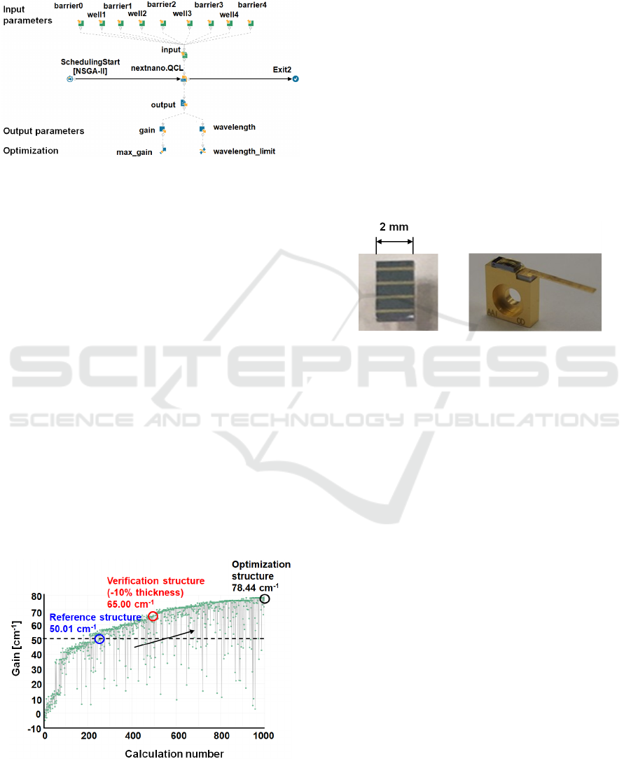
4 SIMULATION RESULTS

Figure 7 shows the modeFRONTIER setting screen

showing the flow of calculation. The upper row

shows the input parameters, the middle row shows the

nextnano.QCL calculation, and the lower row shows

the output items. The input parameters correspond to

the nine film thicknesses shown in Table 1. The nine

film thicknesses of the injector barrier and active

region were inputted into nextnano.QCL, and the gain

and wavelength for each film structure were

Optimization of Active Region of Quantum Cascade Laser (QCL) by Coupled Calculation of Genetic Algorithm and QCL Simulator

calculated. On the basis of the gain, the next-

generation parameter set was obtained using the GA

described in Section 3.2, and the process of

optimization proceeded.

Figure 7: Setting screen of modeFRONTIER for

optimization of active region in QCL.

To examine the effect of optimization by

experiments, we added the reference structure

reported previously (Evans et al., 2007) and the

verification structure in which all film thicknesses

were reduced by 10% to the optimization

calculations. The reason for reducing the film

thickness of each layer by –10% was that such a film

can be deposited by shortened MBE process time and

the desired film structure can be reliably produced.

Figure 8 shows the results of the coupled

calculation of nextnano.QCL and genetic algorithm.

The horizontal axis shows the number of calculation,

and the vertical axis shows the gain of the structure

corresponding to the calculation number. As the

generation of genetic algorithms increases, the gain

increases.

The reason why the gain intermittently decreases

during optimization is that the mutation conditions for

the GA were calculated and some of them showed

low gains. As a result, while the gain of the reference

structure was 50.01 cm

–1

, that of the verification

Figure 8: Progress in optimization by coupled calculation

of genetic algorithm and QCL simulator.

structure was as high as 65.00 cm

–1

. Furthermore, in

the final structure, a gain of 78.44 cm

–1

was obtained,

and it was estimated that high-power laser oscillations

can be obtained.

5 EVALUATION OF

OPTIMIZATION RESULTS

To examine the validity of the optimization

calculations, we fabricated prototype devices with the

reference and verification structures, and we

examined the EL light output. Figure 9(a) shows a

photograph of external the prototype QCL chip. The

injector and active regions, which contribute to light

emission, were stacked 33 times, and the chip had a

length of 2 mm and a ridge width of 100 µm.

(a) (b)

Figure 9: Photograph of prototype QCL. (a) QCL chip with

length of 2 mm and ridge width of 100 mm, and (b) QCL

device soldered on CuW mount.

Figure 9(b) shows a QCL device soldered on a

CuW mount. The device was cooled to 77 K and

operated at a frequency of 100 kHz and a pulse width

of 300 nm (3% duty). The emitted light was focused

by a concave mirror, and the EL intensity was

measured by an MCT (HgCdTe) detector.

Nicolet8700 (ThermoScientific Inc.) was used to

measure the EL spectra.

Figure 10 shows the EL spectra of the prototype.

The horizontal axis represents the wavelength and the

vertical axis represents the EL emission intensity. A

strong luminescence was observed for both the

reference and verification structures. The oscillation

wavelengths of the reference and verification

structures were 4.53 μm and 4.77 μm, respectively.

Here, in the simulation results in Section 4, the

wavelengths of the reference and verification

structures were 4.77 nm and 4.93 nm, respectively.

For both film structures, the experimental results

had shorter wavelengths than the simulation results.

However, in both experiments and simulations, the

wavelengths of the verification structure were longer

than those of the reference structure. The trend in the

two types of structure was consistent in experiments

PHOTOPTICS 2024 - 12th International Conference on Photonics, Optics and Laser Technology

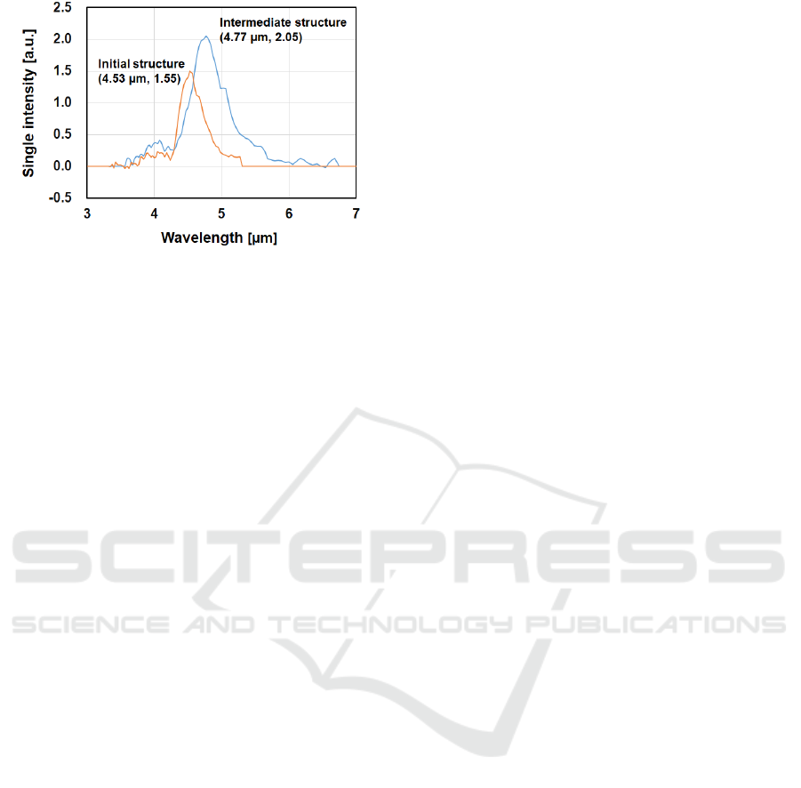
Figure 10: EL emission intensity of prototype QCL device

(Tanimura et al., 2022).

and simulations. Corresponding to the gain of the

optimization calculation, the emission intensity of the

verification structure was 1.37 times higher than that

of the reference structure. From these results, it is

estimated that the structure optimized using the gain

in the optimization simulation can have a higher

emission intensity than the reference and verification

structures.

6 CONCLUSIONS

We applied a coupled calculation of genetic algorithm

and the QCLsimulator (nextnano.QCL) to calculate

the gain that excites laser light in the active region of

the QCL. The thicknesses of the nine layers

constituting the active region were changed

simultaneously, and the film structure with the

maximum gain was determined from 1000 types of

the parameter sets.

Nextnano.QCL incorporating a non-equilibrium

Green's function was used to calculate the gain of

QCL, and the validity of the simulation was evaluated

using the active region structure reported previously

(Evans et al., 2007). In the coupled calculation of

genetic algorithm and nextnano.QCL, we used gain

as an objective function and used the methods of

crossing, natural selection, and mutation simulating

the evolutionary process of living organisms to

optimize the nine film thicknesses in the active

region. As a result of the optimization calculation, the

optimized structure had a gain (78.44 cm

–1

) higher

than that (50.01 cm

–1

) in the structure reported in a

previous paper.

In addition, as a result of prototyping the QCL of

the reference and verification structures and

measuring the EL emission, the emission intensity of

1.37 higher than that of the literature structure was

obtained for the verification structure, demonstrating

the validity of the optimization.

ACKNOWLEDGEMENTS

This work was supported by Innovative Science and

Technology Initiative for Security, ATLA, Japan.

REFERENCES

Faist, J., Capasso F., Sivco D. L., Sirtori C., Hutchinson A.

L., & Cho A. Y., 1994. “Quantum cascade laser”,

Science, 264, 553–556.

Faist J., Villares G., Scalari G., Rösch M., Bonzon C., Hugi

A., & Beck M., 2016. “Quantum Cascade Laser

Frequency Combs”, Nanophotonics, 5, 272–291.

Lu S. L., Schrottke L., Teitsworth S. W., Hey R., & Grahn

H. T., 2006. “Formation of electric-field domains in

GaAs⁄AlxGa1−xAs quantum cascade laser structures”,

Phys. Rev. B, 73, 033311.

Grange, T., 2015. “Contrasting influence of charged

impurities on transport and gain in terahertz quantum

cascade lasers”, Phys. Rev. B, 92, 241306-1–5.

Tanimura H., Takagi S., Kakuno T., Hashimoto R., Kaneko

K., & Saito S., 2022. “Analyses of Optical Gains and

Oscillation Wavelengths for Quantum Cascade Lasers

Using the Nonequilibrium Green’s Function Method”,

Journal of Computer Chemistry, Japan-International

Edition, 8, 2021–0024.

Evans, A., Darvish, S. R., Slivken, S., Nguyen, J., Bai, Y.,

& Razeghi, M., 2007. “Buried heterostructure quantum

cascade lasers with high continuous-wave wall plug

efficiency”, Appl. Phys. Lett. 91, 071101.

Takagi S., Tanimura H., Kakuno T., Hashimoto R, & Saito

S., 2021. “Evaluation of Simulator Incorporating Non-

equilibrium Green’s Function and Improvement of

Quantum Cascade Lasers Output using the Simulator”,

Proceedings of PHOTOPTICS 2021, 58–63.

Holland J. H., 1975. “Adaptation in natural and artificial

systems: an introductory analysis with applications to

biology, control, and artificial intelligence”, University

of Michigan Press.

Holland J. H., 1992. “Genetic Algorithms”, Scientific

American, 267, 66–73.

Takagi S., Sekine M., Nakaegawa T., & Hsiao S.-N., 2023.

“Optimization of RF Frequencies in Dual-Frequency

Capacitively Coupled Plasma Apparatus Using Genetic

Algorithm (GA) and Plasma Simulation”, IEEE Trans.

Semicond. Manuf., 36, ,547–552.

Debi K., Pratap A., Agarwal S., & Meyaraivan T., 2022. “A

Fast and Elitist Multiobjective Genetic Algorithm:

NSGA-II”, IEEE Trans. Comput., 6, 182–197.

Optimization of Active Region of Quantum Cascade Laser (QCL) by Coupled Calculation of Genetic Algorithm and QCL Simulator