Finite Interval Processes: Simulating Military Operations

Robert Mark Bryce

Defence Research and Development Canada (DRDC) – Centre for Operational Research and Analysis (CORA),

Keywords:

Stochastic Process, Military Operations, Scheduling.

Abstract:

We discuss extending Poisson point processes to ﬁnite interval processes, in the context of simulating military

operations over time. Conceptually the extension is simple, points are extended to ﬁnite duration of length

equal to the operations’ duration. We discuss effects of ﬁnite duration, namely lowering of set frequencies (and

therefore artiﬁcially reduced expected demand) due to the extension of points to intervals—and its correction.

The Canadian Armed Forces (CAF) has a Force Structure Readiness Assessment (FSRA+) Monte Carlo sim-

ulation tool that implements a ﬁnite interval process, and the results here offer insight on the approach.

1 INTRODUCTION

Armed Forces project military power via operations,

and the capacity to maintain operations is fundamen-

tal to delivery a credible military capability. As one

example, the Canadian Armed Forces (CAF) is man-

dated under the Canadian Defence strategy Strong,

Secure, Engaged (SSE) (Department of National De-

fence, 2017) to deliver concurrent operations of speci-

ﬁed attributes including location (domestic or interna-

tional), size, and duration. The purpose of this paper

is to consider modelling operations as a ﬁnite interval

stochastic process, which is derived from a stochas-

tic point process model, to support analysis of mili-

tary operations over time (e.g., to estimate mat

eriel—

including ammunition—usage, determine stafﬁng re-

quirements, etc.).

The CAF has developed an approach (Force Mix

Structure Design, or FMSD) and a related Monte

Carlo tool (Force Structure Readiness Assessment, or

FSRA+) which considers operations occurring over

time. The main focus of the approach is currently

on stafﬁng (Dobias et al., 2019), but is general and,

for example, mat

eriel usage can be considered (Serr

2021). As operations have various Force Elements as-

signed to them, for example, a Field Artillery Battery,

Field Hospital, or Frigate, given this mapping analy-

sis can make use of this reﬁned level of detail. A good

overview of the development and use of FSRA+ is

provided by (Dobias et al., 2019), which is a key rele-

vant publication describing ﬁnite interval processes to

model military operations. For our purposes we will

strip down to a simpliﬁed version of FSRA+, where

we do not consider concurrency and other compli-

cating factors which FSRA+ accounts for, and rather

we solely consider the scheduling of operations of set

types over a time horizon. The core parameteriza-

tion of operations is a label (allowing identiﬁcation

which allows, for example, observing which opera-

tions occur when and for Force Elements to be as-

signed), a probability distribution describing an oper-

ations’ durations (currently a triangular distribution is

being used by FSRA+), and an annual frequency of

occurrence. To create a realization a time horizon is

set (e.g., 5 or 10 years), time is discretized into time

steps ∆t (e.g, 1 or 2 months), and, starting from t = 0,

the time steps are stepped through and operations are

either started, or not. To determine if an operation is

initiated in a time step the following heuristic method

is used (Strategic Analysis Support, 2019). A pool of

candidate operations is made by drawing K

copies of

the ith operation, using the relevant Poisson parameter

describing the frequency of occurrence. This pool can

be empty, or ﬁlled with various copies of operations.

The pool is then drawn from, uniformly at random.

The operation type drawn, if any, is then initiated, a

duration drawn, and the next time steps ﬁlled with the

operation. The process then steps to the next time

step and proceeds until the time horizon is exhausted.

To mitigate initial condition artifacts there is a burn-

in period, equal to the time horizon length, which is

truncated. This approach is pragmatic and has been

subject to empirical tests. We note the following—

the heuristic approach closely follows the continuous

356

Bryce, R.

Finite Interval Processes: Simulating Military Operations.

DOI: 10.5220/0012424700003639

Paper copyright by his Majesty the King in Right of Canada as represented by the Minister of National Defence

In Proceedings of the 13th International Conference on Operations Research and Enterprise Systems (ICORES 2024), pages 356-363

ISBN: 978-989-758-681-1; ISSN: 2184-4372

time Poisson process and the related Bernoulli pro-

cess (the discrete time approximation), where there

is slight differences in sampling (e.g., the pool) and,

instead of single time step durations, extended ﬁnite

durations are considered. Here will look at the con-

tinuous time Poisson point process and extending it

to a ﬁnite interval process to allow more direct con-

tact with the Poisson point process.

Details are provided in the theory section, but in

brief we sample independent realizations from Pois-

son point processes parameterized by the initiation

frequencies of the various operation mix we are mod-

elling, merge these, and then expand by sampling du-

rations. When moving from a point process, where

there is no duration (inﬁnitesimals), to ﬁnite inter-

vals there is an expansion of the time axis (see Fig-

ure 1). This expansion will result in realizations of

the stochastic process to have observed frequencies

lower than the set input frequencies, which will have

a corresponding reduction in the demand. This ef-

fect can be pronounced, depending on the frequency

and the durations. For example, if one has an annual

frequency (1/year) and a ﬁxed duration of one year

then after expanding the observed frequency will half

thereby leading to a signiﬁcant effect. The effect of

frequency reduction will be to reduce the observed

frequency of a given operation type, biasing analy-

sis in a manner which can be signiﬁcant. A core aim

of this paper is to qualify and quantify this frequency

reduction.

Figure 1: Expansion when moving from a point to an in-

terval process. The ﬁnite durations expands the time scale,

reducing the operational frequencies.

This paper proceeds as follows. We ﬁrst sketch

the required theory, outlining the approach taken in

more detail. We then describe the frequency reduc-

tion seen in the input operation frequency due to ﬁ-

nite durations (expansion) and develop a correction.

We next provide a scheme to remove initial condition

artifacts to ensure ergodicity before overviewing the

algorithmic approach taken. We then outline numer-

ical experiments to subject our theory to test and in

the results section we provide the numerical evidence

to allow assessment of the approach developed here.

In the discussion we consider implications and future

work, before concluding.

2 THEORY

2.1 Finite Interval Processes:

Continuous Time

A Poisson process can be considered as time ordered

points (inﬁnitesimals of zero measure) that are sep-

arated by exponentially distributed intervals λe

−λt

where the rate λ parameterizes the distribution. Of

importance here, Poisson processes are additive so

if we have two processes X ∼ Poisson(λ

) and Y ∼

Poisson(λ

) then X +Y ∼ Poisson(λ

+ λ

) (see, for

example, (Gallager, 2013)). If we have two realiza-

tions, X and Y , which have points at speciﬁc times,

we can simply combine (merge) these to obtain a re-

alization of the combined process.

Here we will take the following stance: we will

make use of the tractability and core understanding of

the Poisson point process as the foundation to build

on. We will determine operation start times using

Poisson process realizations, for each operation type

or variant we consider. We then use their additive

properties to merge them together (here we note that

formally, as the points are real numbers, we have zero

probability of collision when we merge). After merg-

ing we then turn the point process into an interval

process, by sampling the appropriate duration distri-

bution and expanding time by these durations in a for-

ward manner (e.g., we start with the ﬁrst instance and

expand—moving each subsequent point to the right—

and work through each point; see Figure 1). One de-

tail: each of our processes have their ﬁrst point occur

after t = 0, e.g., we do not start on, or in, an operation.

This implies there will be initial time artifacts, which

we will address below.

In summary, we rely on the additive property of

Poisson processes to allow independent realizations

(each describing an operation of a given type) to be

combined, and then turn this into a ﬁnite interval pro-

cess by expanding by the appropriate durations. In-

trinsic to the process we will have a reduction of set

input frequencies, as we expand time by the durations.

2.2 Frequency Reduction

Here we consider the frequency reduction of a point

process as it becomes a ﬁnite interval process.

Consider a single operation of type, or variant, i.

The average case will have mean duration

and, for

point processes, there is a typical separation of T

1/ f

, where f

is the set frequency. The intention is

that the time between operation starts is, on average,

, but instead the observed time between operations,

, is inﬂated by the ﬁnite duration of operations

Finite Interval Processes: Simulating Military Operations

357

+ d

1 + f

, (1)

where

is the observed frequency.

We can artiﬁcially increase the input operations’

frequency such that, after expansion, will recover the

desired frequency, as follows

1 − f

(2)

which can be conﬁrmed by substituting back in Equa-

tion 1 which recovers the intended

= 1/ f

. Note

that we have the requirement that f

is strictly less

than one.

The frequency reduction, and its correction, can

be understood by considering the amount the unit

time expands when we move from a point process to

an interval process. In expectation, for the single vari-

ant case, we have f

expansion per unit time, and so

to correct this we have to rescale by 1 − f

. This

indicates that for the multi-variant case we want to

rescale by the total expansion and so

1 −

∑

, (3)

and now our constraint is that

∑

must be strictly

less than one. If this condition cannot be met then we

cannot correct.

As an example of frequency reduction and its’ cor-

rection consider two variants, both with a frequency

of 0.1/year and a mean duration of 2.5 years. In ex-

pectation, for point processes on 10 year horizon we

expect one of each variant and so will see an expan-

sion to 15 years, dropping their observed frequency

to 1/15. If we apply the correction we ﬁnd

= 1/5,

a signiﬁcant change from the desired 1/10 frequency.

In expectation, for such point processes on a 5 year

horizon we expect one of each variant and we see an

expansion to 10 years—we will observe the desired

frequency of 0.1.

To summarize, if we use the set frequencies for

operations of ﬁnite duration we will see an expansion,

which has the effect of initiating fewer operations of

a given type per unit time then intended. If

∑

is one or greater we cannot correct this situation and

our proposed operations and their parameters are mis-

speciﬁed and our assumed model is not realizable—if

we want to take the na

ıve view that input frequencies

describe the operations frequency. If

∑

is less

than one, then we can correct by applying Equation 3

to our set (intended) frequencies and use these when

making realizations of our stochastic process.

2.3 Initial Condition Artifacts

As operations start at t > 0 we cannot start mid-way

through an operation. This means that ergodicity is

violated, as the initial time region is special due to

initial condition artifacts. To correct for this we can

truncate the ﬁrst part of a simulated time line, a pro-

cess known as burn-in. For example, recall FSRA+

takes a pragmatic view of doubling the time horizon

and truncating the ﬁrst half to mitigate initial condi-

tion artifacts.

Here we propose an alternative approach. We

build up operations which occur some time after t

0 and which end at some maximum time, t

= M, at

the termination of the last operation. We consider

time to be periodic (i.e., t

= t

and time “wraps

around”). If we uniformly, at random, select a point in

[0,M) and set this as the new t

we will no longer priv-

ilege any time. The expected probability of starting

with t

in an operation is the mean duration divided by

the expanded unit time (i.e.,

∑

/(1 +

∑

)),

and we see that our uniform selection of a start time

in our simulated time horizon will cut an operation

with the same probability—our randomized start time

procedure will ensure ergodicity and eliminate initial

condition artifacts.

2.4 Overview of the Core Algorithm

We now review the core concepts of the algorithm:

1. For each operation type (variant) we sample the

appropriate exponential distribution to ﬁnd inter-

operation distances such that we cover the simu-

lation interval T , and the appropriate distribution

paramaterization to ﬁnd durations. We ﬁnd the

start times for the point process.

2. We merge these processes, retaining order by start

time.

3. We expand, using the durations. We truncate at

the end of the last operation instance.

4. We randomly select a start time with periodicity

in mind, enforcing ergodicity.

The inputs required are the desired simulation time

horizon T , the scenario’s frequencies, and the sce-

nario’s duration parameterization. The output is a

table/dataframe with operation type id’s, start times,

and durations over a simulated time that is ≳ T long.

Depending on analysis one either can truncate at T ,

or retain the longer horizon to improve statistics (here

we do not truncate).

Note that, to correct for expansion effects (in-

put frequency reduction), the operations’ frequencies

ICORES 2024 - 13th International Conference on Operations Research and Enterprise Systems

358

should be increased according to Equation 3 and these

be used.

3 NUMERICAL EXPERIMENTS

We consider several special cases and numerical ex-

periments to verify the theory and discuss practical

concerns. The intent is not an exhaustive study, but

rather to subject the core elements to critical tests.

3.1 Case 1: Single Variant

The simplest case is a single operation.

Case 1: We consider a set average frequency of

once a year and uniformly distributed durations on

[0,2(1 −ε)) so that the average duration is d = 1 −ε.

Inverting Equation 1, we ﬁnd the expected fre-

quency reduction is

f = 1/(2 − ε); as a check on

the theory, note that for ε = 0 the average duration

is one and so we expect the frequency to half and as

ε → 1 we converge to a point process and expect no

frequency reduction (frequency remains unity). The

frequency correction is

f = 1/ε.

We will measure the observed reduction in fre-

quency as a function of ε and compare against the the-

ory. Additionally, we will perform the correction as a

function of ε and observe the frequency and compare

against expectation (unity).

3.2 Case 2: Multiple Variants

We consider multiple operation types. For simplicity

we will consider ﬁxed duration.

Case 2: Here we consider a ﬁxed duration of one

year, and a frequency of 1/2

where i indexes the op-

erations. In the limit of inﬁnite operations we there-

fore have

∑

→ 1 and we approach the

singularity in a controlled manner.

Here we will perform the correction and mea-

sure the normalized residual. Our set (intended) fre-

quencies are f

= 1/2

and the correction is

(1/2

)/(1 −

∑

j=1

(1/2

), where we have K variants

(in the limit of K → ∞ we hit a singularity). It can be

shown (via induction) that

∑

j=1

(1/2

) = (2

−1)/2

and so we ﬁnd

= 2

K−i

. We apply the correction,

run our numerical experiments, and observe the fre-

quencies

and compare with the intended frequency

= 1/2

. To summarize the error we look at the

summed absolute normalized residual R

∑

−

1/2

|/(1/2

), which we expect to have a positive bias

(as we are taking the absolute values and summing).

We will look at various K, and plot R

against 1/K

such that as K → ∞ we have 1/K → 0 and we can

plot on (0,1].

3.3 Case 3: Ergodicity

We consider our proposed means of ensuring ergod-

icity and eliminating initial condition artifacts.

Case 3a: We consider a single operation type,

where have a set frequency of 0.1/year and a symmet-

ric triangular distribution with a minimum duration of

0 years, a mode of 1 year, and a maximum of 2 years

(average duration of 1 year). We will experimentally

measure how often we cut an operation when select-

ing our new t

, and compare it against the expected

value of 1/(10 + 1) = 0.09.

Case 3b: We consider the multi-operation type

case, with two variants. The ﬁrst is parameterized as

in Case 3a and the second has twice the frequency

and duration. We again experimentally measure how

often we cut operations when we select our new t

here tracking which variant is cut. The expected value

of cutting an operation is 0.1/(1 + 0.5) + 0.4/(1 +

0.5) = 1/15 +4/15 = 1/3 = 0.3, where the ﬁrst term

is the probability of cutting the ﬁrst operation type

(1/15 = 0.06) and the second term is the probability

of cutting the second operation type (4/15 = 0.26).

4 RESULTS

4.1 Case 1: Single Variant

We simulate over a time horizon of 100,000 years and

we replicate this 100 times. In Figure 2 we see that

the derived frequency reduction (solid line) accurately

describes the observed frequencies (dots). Stochastic

ﬂuctuations are smaller than the symbol size (standard

deviations are on the order of 10

−3

Figure 2: Observed (dots) and theoretical (line) frequency

reduction for Case 1.

We then ﬁrst apply the frequency correction and

then simulate. To prevent hitting the singularity we

Finite Interval Processes: Simulating Military Operations

359

use a minimum ε of 0.01 in place of zero. Figure 3

demonstrates that the correction results in the recov-

ery of the desired frequency (unity here). The error

bars illustrate the standard deviations observed.

Figure 3: Observed (dots) and expected (dotted line) fre-

quency, when frequency correction is applied for Case 1.

4.2 Case 2: Multiple Variants

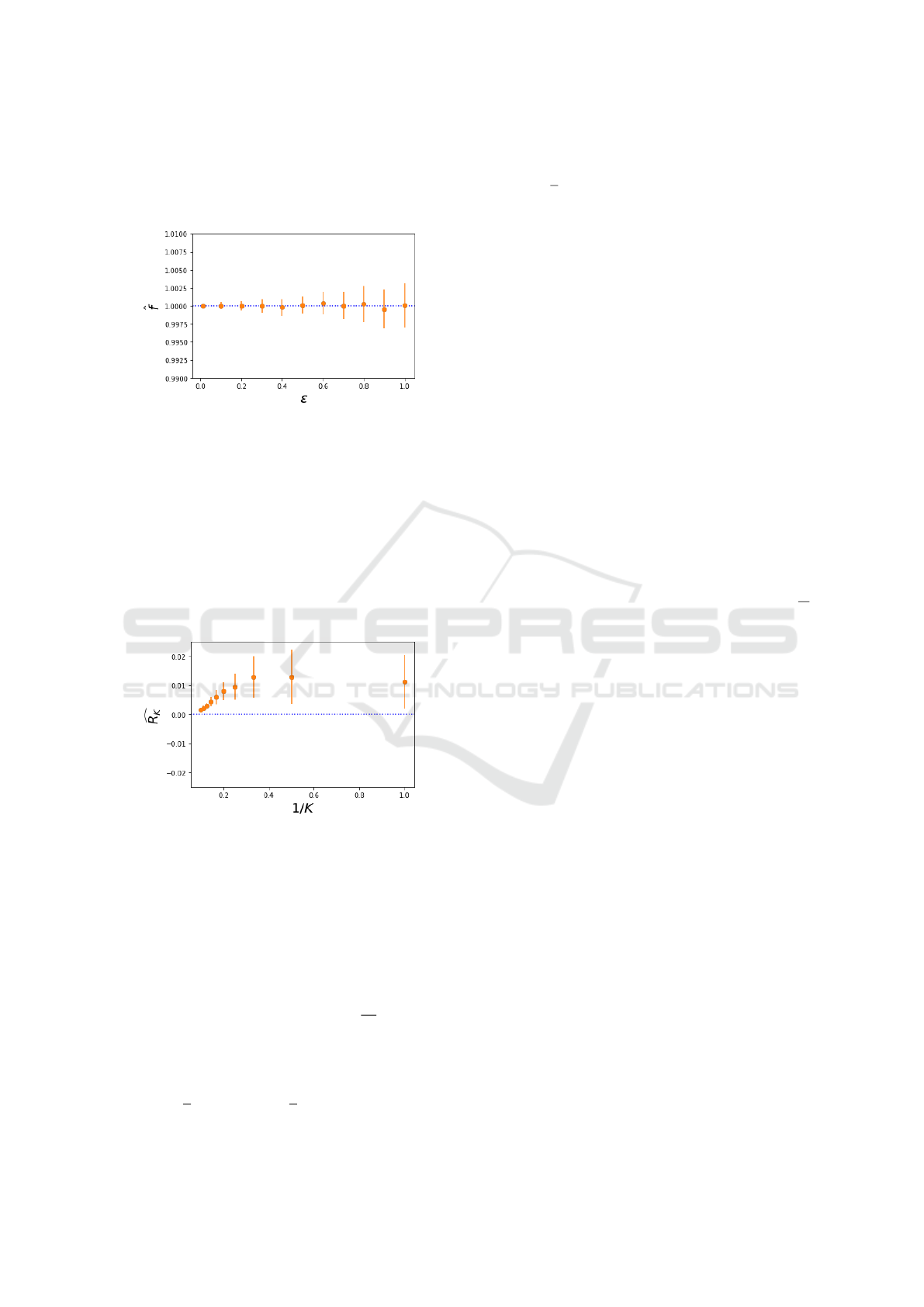
Here we consider a time horizon of 1,000 years and

100 replications. We look at K = 1 . ..10 and ﬁnd the

summed absolute normalized residual R

of the fre-

quencies. We see limited error in Figure 4, e.g., at low

K we see about 1% error, and as K →∞ both the error

and variance (error bars are the standard deviations

observed) appear to converge to zero.

Figure 4: Observed (dots) and expected (dotted line) nor-

malized residual, when frequency correction is applied for

Case 2.

4.3 Case 3: Ergodicity

For Case 3a (single variant) we consider a time hori-

zon of 1,000 years and 10,000 replications. We ﬁnd

that the observed probability of cutting an operation

(having t = 0 selected to start within an operation)

to be 0.0933, with a standard error of 0.00291—in

agreement with the expected value of 0.09.

For Case 3b (two variants) we ﬁnd for the ﬁrst

(second) operation the probability of a cut is 0.0671

(0.262) with a standard error of 0.00250 (0.00440)—

again in agreement with the expected values (of

1/15 = 0.06 and 4/15 = 0.26); the probability of cut-

ting any operation is 0.329 with a standard error of

0.00470, in agreement with the overall expected value

of 1/3 = 0.3.

5 DISCUSSION

For both Case 1 (single variant) and Case 2 (multi-

ple variants) as the magnitude of the frequency cor-

rection becomes large (ε → 0; K → ∞) the error be-

comes small (see Figure 3 and 4); for both cases we

see variation reduce signiﬁcantly and error trend to-

wards zero. We attribute this to reduced ﬁnite sample

size induced variation and error (law of large num-

bers): note that as the correction becomes large we

have higher frequency, and so we will have both less

sampling variation and smaller overall error. The

larger apparent error in Case 2 over Case 1 can be at-

tributed to two factors. First, use of a shorter horizon;

computational time was much longer for equivalent

time horizons in Case 2 over Case 1, which can be at-

tributed to the overall 55 more variants considered (as

we range K from 1 to 10) and so a shorter time hori-

zon was selected. As the time horizon is 100X shorter

than in Case 1 we expect roughly 10X the ﬁnite sam-

ple induced error over Case 1 (following the ∝ 1/

√

rule for the standard error of the mean, where N is the

sample size)—however, note that in Case 1 we have

stochastic durations while in Case 2 we ﬁx our dura-

tion that source of error is eliminated in Case 2, which

is a mitigating factor. Second, in Case 2 we look at the

summed absolute normalized error so absolute values

are taken in Case 2, rather than the mean frequency in

Case 1 (where ﬂuctuations will tend to average out),

and so error is nonnegative and additive.

For context in interpreting the error levels ob-

served in Case 2, note that for lower K values we

see we have a relative error level of 1%—compare

this to the frequency reduction expected for an uncor-

rected input frequency of roughly 30% relative error

for K = 1 (as 1/2 shifts down to 1/3).

For K = 10 we expect, on average, less than one

operation per realization for the 10th operation and

here we ﬁnd the total absolute error is larger (0.00160,

with a standard mean error of 0.0000525), but on the

order of, the error associated with that term alone

when we have no operation (1/2

≈ 0.001)—we are

seeing limited, ﬁnite sample based ﬂuctuations. It is

worth mentioning that as 1/K → 0 we have ﬁrst mod-

erately increasing, and then more strongly decreasing,

error. We attribute this to two competing effects (in

addition to the visual artifact whereby the decreasing

separation of points on the 1/K axis makes the slope

appear larger). First, the above mentioned law of

ICORES 2024 - 13th International Conference on Operations Research and Enterprise Systems

360

large numbers suppressing ﬁnite sample induced er-

ror. Second, as K increases we have more terms in the

residual sum and thus increasing error (note, however,

that the rate of growth of the sum rapidly decreases as

more terms are added). These two effects will com-

pete and we attribute the complex shape to this com-

petition. Future work can increase the time horizon or

replication number to drive the error levels lower and

increase precision, and could also break away from

the summed absolute error, which was selected as a

simple summary statistic at a cost of magnifying ob-

served error, to look at individual

components—

however, the results here are strong and provide quan-

titative support of the frequency correction efﬁcacy.

We ﬁnd that ergodicity holds following our initial

time selection scheme, in the sense that we start time

(select our t = 0) in the midst of an operation with the

expected probability for the cases we checked. We

expect this, as our merged process, as long as it holds

at least one operation, will consist of inter-operation

separations and operations without any truncation ef-

fect (recall that we start at t = 0 and end at a maximum

time t

= M at the termination of the ﬁnal operation).

If we then randomly select a point in [0, M) as our new

t = 0 we will cut operations with the correct probabil-

ity, by design. The result is there is no privileged time

and ergodicity holds.

In this work we considered continuous time,

where we take a point process and extend to a ﬁnite

interval process. This expansion results in reduction

of operations’ frequencies from those used as input.

While we do not consider the discrete time approx-

imation we note that the FSRA+ approach iterates

through the discrete time steps, and when we initi-

ate a operation we draw a duration and ﬁll in that

many time steps before proceeding. So we see the

frequency reduction also occurs in the discrete time

step approximation approach, which is intuitive as

our initiation probability assumes we draw on each

time step yet skipping/expanding over several time

steps for ﬁnite durations reduces the initiation fre-

quency. If one desires a discrete time output, for

example for analysis purposes, creating a continuous

time realization followed by discretization is an op-

tion, as is use of FSRA+ which directly uses discrete

time. Additionally, inspired by FSRA+ and the work

here, a slightly modiﬁed approach has been outlined

in (Bryce, 2023), and which is summarized in the

Appendix: Synopsis of a discrete time algorithm to

schedule military operations.

We note that the pool sampling used by FSRA+

to initiate operations is heuristic, and therefore there

is some concern that it may introduce error. Here we

elucidate biasing effects and provide some evidence

that any bias will be small, by considering the sim-

plest case: two variants, say of type x and y. For the

two variant case, the pool process will lead, in a given

time step, a relative probability of an operation of type

x of

′

= X/(X +Y ), however note that

E[p

′

] = E[X /(X +Y )] ̸= E[X]E[

X+Y

]

̸=

E[X]

E[X+Y ]

E[X]

E[X]+E[Y ]

+λ

(4)

where we desire the left side be equal to the right

side to obtain the correct relative probability p

′

, but

as the numerator and denominator are not indepen-

dent we have the ﬁrst inequality and due to Jensen’s

inequality we have the second inequality (see, for ex-

ample, (Wasserman, 2004)), and the left hand and

right hand sides are not strictly equal in general.

However, note that the ﬁrst effect tends in one di-

rection (as the covariance of X and 1/(X + Y ) is

negative; recall that E[AB] = E[A]E[B]+Cov(A,B))

while the other effect is in the opposite direction

(E[1/A] > 1/E[A]) and so they will tend to cancel

each other. Further, note that p

′

+ p

′

= 1 must hold

and so the bias sign and magnitude is sensitive to

the parameters; if one is biased in one direction the

other must be biased in the other direction. Numeri-

cal experiments show that bias is small for even rel-

atively large separation in parameters. For example,

for λ

= 1 and λ

= 99 we sample a billion X and

Y Poisson numbers (near the memory limit of the

machine used), ﬁnd

′

and

′

, and repeat this 100

times: the mean values are 0.00999998970013 with

a standard error of 0.00000000000978 (expectation

is 0.01) and 0.99000001029986 with a standard er-

ror of 0.00000000000978 (expectation is 0.99). We

see a small (negligible), but existing, bias. While the

arguments here are on the simpler case of two vari-

ants the insights should apply to larger numbers of

variants (for example, if we group and label all op-

erations not of type x as y the arguments here hold,

and much of the insight can directly apply to more

than two variants). To quantify the magnitude of any

bias it would be useful to test with the speciﬁc oper-

ations mix and parameterizations modelled, however

the arguments here provide a qualiﬁed veriﬁcation of

the pool heuristic, as any bias will be small due to

the competition of the biasing effects and the small

magnitude observed even for relatively large parame-

ter differences in the two variant case (the considered

parameters of 1 and 99 speaks to a ≈ 100 fold differ-

ence in frequency, which should capture the parame-

ter range seen in many contexts). The pool sampling

heuristic appears to perform well in practice.

To keep focused on essentials we have not consid-

ered concurrency constraints here, however this con-

sideration is important in practice so we will provide

Finite Interval Processes: Simulating Military Operations

361

some comments. First, one can not constrain con-

currency by sampling start of operations via realiz-

ing a Poisson process and determine their ends by

sampling the appropriate duration distribution (here

time is not expanded, rather operations are overlaid

on the time axis). This approximation can be suitable

(see, for example, (Fee and Caron, 2021) or (Couil-

lard et al., 2015), where this approach is used in a

military context, and the references within) and does

not suffer from frequency reduction, but, in general,

we can have an unbound number of concurrent op-

erations if we use this approach and so peak concur-

rency can be unrealistic. Second, using the ﬁnite in-

terval process approach allows us to simulate a man-

date to have C concurrent operations by considering C

parallel independent realizations, where each realiza-

tion has appropriately scaled frequencies ( f

→ f

/C ).

The additive property of Poisson processes will led to

the correct overall frequency for each operation type

when we take the C parallel realizations in combina-

tion, and we see that by considering C parallel realiza-

tions we allow up to C concurrent operations. More

generally, we may have lines of operation, each of

which with relevant operation types and concurrency

requirements and we would break the simulated time

line out to determine the overall realization (for exam-

ple, SSE mandates two major sustained deployments,

one major time-limited deployment, two minor sus-

tained deployments, and two minor time-limited de-

ployments, as well as other requirements (Department

of National Defence, 2017)). It is noteworthy that

FSRA+ does account for these lines of operations and

concurrency requirements, as well as other complex-

ities such as ongoing constant demands and various

constraints on Force Elements (Dobias et al., 2019).

FSRA+ speaks to the capacity and capability of

the CAF, and breaks down operations by Force Ele-

ments and stafﬁng of those Force Elements. For this

reason FSRA+ lives on a classiﬁed network. The op-

eration variants and scheduling parameterizations are

not secret, as the underlying information is available

in the public domain, and so schedules themselves are

not classiﬁed. One motivation of this work was to

work towards a light weight operation schedule gener-

ator which could be used off the classiﬁed network, to

facilitate analysis (e.g., in the study (Serr

e, 2021) only

schedules output by FSRA+ where used and analysis

was done off the classiﬁed network). Due to suitabil-

ity for development and analysis Python was selected

as a language, which makes time stepping computa-

tionally expensive, which was a pragmatic rationale

for considering continuous time processes (however,

see the Appendix for a discrete time approach that is

viable in Python). On the formal side, making con-

tact with established theory and basic principles was

a key motivator and rationale for considering con-

tinuous time. The results here lay the ground work

for a more mature implementation that can simulate

CAF operation schedules, taking line of operations

and concurrency into account.

While we have focused on scheduling of military

operations, as this was the application in mind, un-

scheduled maintenance and other such applications

can be addressed with the same approach. For ex-

ample, unplanned air craft maintenance schedules can

be generated, given a mixture of maintenance types

(“operation types”), their frequency, and the number

of aircraft (“concurrency”), and with these schedules

resource use can be determined.

Two key aspects have been established here. First,

we provide an independent validation of the FSRA+

approach by making contact with stochastic processes

and, second, in doing so provide a scheme to ensure

input frequencies are recovered. This is important as

it simpliﬁes interpretation and as otherwise input fre-

quencies are biased downwards in an opaque manner,

which likewise reduces demands. As a consequence

demands will be lower than suggested by the input

frequencies which implies we will plan for an artiﬁ-

cially small demand.

6 CONCLUSION

Here we extended Poisson point processes to ﬁnite

interval processes, for simulating military operations

over time. The work was motivated by a prag-

matic tool in use by the CAF, FSRA+, which uses

a discrete time approach. We outlined the contin-

uous time approach, characterized the frequency re-

duction whereby input frequencies are reduced when

points are extended to intervals, provided a correction

scheme to address this, provided a scheme to ensure

ergodicity (i.e., eliminate initial condition artifacts,

without the need for burn-in), and subjected the ap-

proach to essential numerical tests. We have also pro-

vided a qualiﬁed veriﬁcation of FSRA+’s pool pro-

cess to initiate operations, demonstrating there will be

a bias—but of small (negligible) magnitude. We note

that the additive property of Poisson point processes is

fundamental in allowing the development and under-

standing of the interval process described here, for ex-

ample allowing concurrency to be cleanly modelled,

which recommends consideration of this approach to

model mixtures of military operations with possible

concurrency mandates.

ICORES 2024 - 13th International Conference on Operations Research and Enterprise Systems

362

REFERENCES

Bryce, R.-M. (2023). Generating military operation

schedules with controlled concurrency: Analysis of

the Force Structure Readiness Assessment approach.

Technical Report DRDC-RDDC-2023-R130, Defence

Research and Development Canada, Ottawa, Canada.

Couillard, M., Arseneau, L., Eisler, C., and Taylor, B.

(2015). Force mix analysis in the context of the Cana-

dian Armed Forces. In Proceedings from the 32nd

International Symposium on Military Operational Re-

search, pages 1–13, Birmingham, United Kingdom.

The Operational Research Society.

Department of National Defence (2017). Strong, Secure,

Engaged: Canada’s defence policy.

Dobias, P., Hotte, D., Kampman, J., and Laferriere, B.

(2019). Modeling future force demand: Force mix

structure design. In Proceedings from the 36th In-

ternational Symposium on Military Operational Re-

search, pages 1–8, Birmingham, United Kingdom.

The Operational Research Society.

Fee, M. and Caron, J.-D. (2021). A simulation model to

evaluate naval force ﬂeet mix. In Kim, S., Feng, B.,

Smith, K., Masoud, S., Zheng, Z., Szabo, C., and

Loper, M., editors, Proceedings of the 2021 Winter

Simulation Conference, pages 1–12, Piscataway, New

Jersey. Institute of Electrical and Electronics Engi-

neers, Inc.

Gallager, R. G. (2013). Stochastic Processes: Theory

for Applications. Cambridge University Press, Cam-

bridge, United Kingdom.

Serr

e, L. (2021). Bridge and gap crossing modernization

project: Modelling the frequency of use. Technical

Report DRDC-RDDC-2021-R082, Defence Research

and Development Canada, Ottawa, Canada.

Strategic Analysis Support (2019). FSRA+ algorithm visual

explanation (slide deck).

Wasserman, L. (2004). All of Statistics: A Concise Course

in Statistical Inference. Springer, New York, New

York.

APPENDIX

Synopsis of a Discrete Time Algorithm to

Schedule Military Operations

We outline a discrete time algorithm to schedule mil-

itary operations, following (Bryce, 2023).

FSRA+ is a single pass discrete time algorithm,

where operations are initiated via a random pool pro-

cess (see the main text for discussion). Figure 5 illus-

trates the creation of a realization. The arrows denote

where operations happen to initiate and colour indi-

cate operation type.

Python was the target language which has the de-

ﬁciency of being computationally slow, making iter-

ation through and modifying vectors detrimental. To

Figure 5: Illustration of operation scheduling, single pass

approach. Figure after (Bryce, 2023).

address this we consider the equivalent two pass ap-

proach where we 1) use a point process to ﬁnd initi-

ation times and 2) expand, as illustrated in Figure 6.

Nominally a two pass approach is worse than a sin-

gle pass, as looping itself and memory operations are

slow in Python, but we can creatively make imple-

mentation choices to mitigate these slow operations.

Figure 6: Illustration of operation scheduling, two pass ap-

proach. Figure after (Bryce, 2023).

In detail, the ﬁrst pass uses the random

choice distribution, drawing ≈ T /∆t numbers

from [0,1,. .., i,...,K] with appropriate probabilities,

where i = 1,. ..,K indicates the ith operation of K to-

tal while zero denotes no operation, T is the nom-

inal time horizon, and ∆t is the discrete timestep.

This can be done using a library (e.g., using NumPy’s

numpy.random.choice), which will be fast. The sec-

ond pass expands by suitable durations where we do

not actually ﬁll in the timeline and expand. Rather, we

take our vector, say v = [0,1,0,0,5,1,0, ...],

and ﬁnd where this is non-zero (in pseudo-code,

idx=which(v > 0)). We then build a table, with

the operation type given by v[idx], start times given

by idx, and suitably drawn durations. We then ex-

pand and makes ergodic via the approach outlined

here, working on the table. This approach accounts

for Python’s characteristic strengths and weaknesses,

and has the advantage of eliminating the identiﬁca-

tion problem where back-to-back operations cannot

be identiﬁed (such as the ﬁnal two operation instances

in Figure 6), which is a concern if counting operations

or if tempo depends on time within an operation.

Finite Interval Processes: Simulating Military Operations

363