Combining Progressive Hierarchical Image Encoding and YOLO to

Detect Fish in Their Natural Habitat

Antoni Burguera

Departament de Matem

atiques i Inform

atica,

Universitat de les Illes Balears, Ctra. Valldemossa Km. 7.5, 07122 Palma, Illes Balears, Spain

Keywords:

Computer Vision, Progressive Image Encoding, Deep Learning, Underwater Robotics.

Abstract:

This paper explores the advantages of evaluating Progressive Image Encoding (PIE) methods in the context

of the speciﬁc task for which they will be used. By focusing on a particular task —ﬁsh detection in their nat-

ural habitat— and a speciﬁc PIE algorithm —Progressive Hierarchical Image Encoding (PHIE)—, the paper

investigates the performance of You Only Look Once (YOLO) in detecting ﬁsh in underwater images using

PHIE-encoded images. This is particularly relevant in underwater environments where image transmission

is slow. Results provide insights into the advantages and drawbacks of PHIE image encoding and decoding,

not from the perspective of general metrics such as reconstructed image quality but from the viewpoint of its

impact on a task —ﬁsh detection— that depends on the PHIE encoded and decoded images.

1 INTRODUCTION

As most existing Autonomous Underwater Vehicles

(AUVs) heavily depend on batteries, their operational

autonomy is limited. This limitation restricts the ex-

ploration of underwater regions to a certain size. To

address this issue, multi-session approaches (Latif

et al., 2013) have been proposed, where extensive

missions are divided into smaller segments, allowing

for recharging between sessions. However, this so-

lution comes with its challenges, including the need

for speciﬁc infrastructure and a signiﬁcant increase

in mission completion time. Consequently, the rele-

vance of multi-robot systems (Do et al., 2020; Bonin-

Font and Burguera, 2020) in underwater environ-

ments is growing. These systems entail deploying

multiple AUVs simultaneously, with each one tasked

to explore a speciﬁc area. This approach ensures

that mission completion time is not compromised, en-

abling the coverage of large underwater areas. Given

the involvement of multiple AUVs, effective commu-

nication becomes essential in these systems.

Underwater communication faces more limita-

tions compared to its terrestrial counterpart (Jaafar

et al., 2022). The attenuation of electromagnetic

waves in water results in reduced bandwidth and lim-

ited transmission distances when using standard Ra-

https://orcid.org/0000-0003-2784-2307

dio Frequency (RF) systems. While acoustic systems

offer larger communication ranges, their bandwidth

typically falls below that of RF. Light-based commu-

nications boast a signiﬁcantly better bandwidth than

both RF and acoustic systems. However, they often

require the transmitter to be in the line of sight of the

receiver, making them susceptible to interruptions due

to water currents, underwater fauna, or unexpected

AUV motions. Consequently, underwater communi-

cation is generally characterized by its unreliability,

slowness, or a combination of both.

While acoustic sensing remains the preferred

modality in sub-sea scenarios, the use of cameras in

underwater robotics has witnessed a signiﬁcant in-

crease in recent years. Numerous studies have delved

into computer vision with an underwater focus (An-

war and Li, 2020), addressing challenges like scat-

tering and poor lighting conditions. These investiga-

tions have successfully facilitated underwater tasks,

including object detection, image segmentation (Bur-

guera et al., 2016), and Visual Simultaneous Localiza-

tion and Mapping (SLAM) (K

oser and Frese, 2020) in

sub-sea environments. This growth in the use of un-

derwater cameras means that image transmission in

multi-robot systems is crucial.

When AUVs share images among themselves or

with a base station, it is important to consider the

communication challenges mentioned earlier. Trans-

mitting raw images or using standard image compres-

Burguera, A.

Combining Progressive Hierarchical Image Encoding and YOLO to Detect Fish in Their Natural Habitat.

DOI: 10.5220/0012423700003660

Paper published under CC license (CC BY-NC-ND 4.0)

In Proceedings of the 19th International Joint Conference on Computer Vision, Imaging and Computer Graphics Theory and Applications (VISIGRAPP 2024) - Volume 4: VISAPP, pages

333-340

ISBN: 978-989-758-679-8; ISSN: 2184-4321

333

sion formats is susceptible to transmission errors or

interruptions in communication. In such cases, Pro-

gressive Image Encoding (PIE) approaches (Monika

et al., 2021; Rubino et al., 2017) come into play. In

essence, PIE algorithms break down the image infor-

mation into chunks, allowing for individual transmis-

sion through the communication medium. The re-

ceiver can then reconstruct the original image, pro-

gressively gaining detail with each received chunk. In

the event of communication loss, the receiver already

has the full image, albeit at a lower quality, and can

seamlessly integrate any remaining chunks once com-

munication is restored.

Well-known examples of PIE include Ordered

Dither Block Truncation Coding (ODBTC) (Guo,

2010), which spatially divides and encodes the image;

Set Partitioning in Hierarchical Trees (SPIHT) (Said

and Pearlman, 1996), which utilizes wavelet trans-

forms for hierarchical partitioning of the image; and

Depth Embedded Block Tree (DEBT) (Rubino et al.,

2017), which combines SPIHT and ODBTC concepts

to improve compression ratio and speed. Some re-

searchers are now introducing the Neural Networks

(NN) into this domain. For instance, (Feng et al.,

2019) employs NN to distinguish relevant objects in

the image from the background, encoding the identi-

ﬁed objects with higher quality.

In the context of underwater robotics, where

specialized software and application-speciﬁc hard-

ware are frequently used, it is desirable for PIE ap-

proaches to be constructed using established algo-

rithms readily accessible through libraries compatible

with diverse hardware platforms and programming

languages. Considering this factor, along with com-

putational efﬁciency and the balance between quality

and size, we devised and published the Progressive

Hierarchical Image Encoding (PHIE) approach (Bur-

guera, 2023; Burguera and Bonin-Font, 2022). This

method hierarchically partitions the image in the color

space, ensuring high quality with a reduced number of

chunks and enabling lossless reconstruction when all

the chunks are received.

To assess PIE approaches, various standard met-

rics, such as the encoding and decoding times, the

evolution of the reconstruction quality with respect

the number of transmitted chunks, or the ﬁnal quality

after receiving all chunks, are commonly employed.

The above mentioned examples excel in some, if not

all, of these metrics. However, it is important to note

that these metrics treat PIE as a general-purpose algo-

rithm, whereas, in reality, these algorithms typically

target speciﬁc applications. For instance, AUVs may

share image data speciﬁcally for Multi-Robot SLAM,

while others may exchange images to build a sea ﬂoor

mosaic or to classify subsea regions based on their bi-

ological or geological structures.

One of these speciﬁc tasks, which is part of the

funded projects PLOME and COOPERAMOS, in

which the author takes part, is that of object detection.

More speciﬁcally, our goal is to detect certain subsea

elements, such as ﬁsh or nephrops and their burrows,

from the images grabbed by a bottom-looking cam-

era endowed on AUVs. Different object detectors are

available in the literature, starting from the early ap-

proaches like Viola-Jones (Viola and Jones, 2001) to

more recent ones like Mask R-CNN (He et al., 2017).

However, even though these methods address speed

and accuracy, they still struggle to achieve standard

video rates, leading to the emergence of one-stage de-

tectors like You Only Look Once (YOLO) (Redmon

et al., 2016).

The YOLO series, ranging from YOLO to

YOLOv8 and including some variants, introduced en-

hancements such as anchor boxes or various train-

ing and inference strategies. Nowadays, YOLO is a

company-backed development model and offers dif-

ferent models ranging from faster and less accurate to

slower and more accurate.

While there are other one-stage approaches like

RetinaNet (Lin et al., 2020) or EfﬁcientDet (Tan et al.,

2020) with unique features, YOLO has become the

de facto standard. The study focuses on YOLO to

perform object detection and, more speciﬁcally, on

YOLOv5 (Ultralytics, ) due to its widespread adop-

tion.

In all these specialized scenarios, including but

not limited to visual object detection, the conventional

metrics evaluating PIE may not accurately capture the

approach’s performance. Therefore, evaluating the

behavior of PIE in the context of their intended tasks

becomes crucial.

In this study, we examine the performance of an

existing PIE approach within the particular ﬁeld of

object detection in underwater environments. To be

more precise, our evaluation focuses on the YOLOv5

object detector when used to detect ﬁsh in their nat-

ural habitat from images encoded using a speciﬁc

PIE algorithm: PHIE. The ﬁndings will demonstrate

PHIE’s effectiveness in progressively encoding im-

ages, not merely from a generic image quality metric

standpoint but from the viewpoint of a highly speciﬁc

and practical application.

VISAPP 2024 - 19th International Conference on Computer Vision Theory and Applications

334

2 PROGRESSIVE IMAGE

ENCODING

The PIE algorithm used in this study is Progressive

Hierarchical Image Encoding (PHIE), which is exten-

sively described, discussed and evaluated with gen-

eral purpose metrics in (Burguera, 2023). Also, the

full PHIE source code, including encoder, decoder

and documentation is available at https://github.com/

aburguera/PHCENCODER. The purpose of this sec-

tion is to overview the algorithm.

PHIE performs recursive clustering of an input

image within the color space, generating a tree struc-

ture known as the PHIE tree. Each tree node under-

goes compression. The process of building the PHIE

tree and compressing each node is called encoding.

The tree can be transmitted node by node, allowing

the recipient to reconstruct the image progressively

upon receiving each node. The process of reconstruct-

ing an image from a PHIE tree, whether complete or

partial, is termed decoding.

Encoding begins by clusterizing the input image

in the color space, resulting in K clusters. Two clus-

terization methods are available in PHIE. The ﬁrst

one, called the Linear Clustering (LC) linearly in-

terpolates K colors, based on their luminance, from

the darkest one to the lightest one in the input image.

The resulting ordered list of K colors is the so called

Color Palette (CP). Then, LC assigns each pixel in

the input image to one of the K clusters depending on

the pixel color proximity to the corresponding color

in CP computed using Euclidean distance in the RGB

space. As a result, each pixel is assigned an index to

CP, building the so-called Cluter Indices (CI).

The second clusterization method, called K-

Means Clustering (KC) uses the well known algo-

rithm K-Means to clusterize the image in the RGB

space. K-Means provides a vector stating the class of

each pixel and the corresponding class centroids. It is

easy to see that these outputs correspond to CI and CP

respectively. Having LC and KC the same input and

output formats, they can be used interchangeably.

Encoding is performed recursively by applying

the same clusterization algorithm to each of the ob-

tained clusters. Recursion ends when the number of

different colors in the input list of pixels is equal or

below K. In this way, the PHIE tree is built where

the root node clusterizes the input image and each re-

maining node clusterizes one cluster of its parent.

Two additional encoding aspects are the follow-

ing. First, after encoding each node the reconstruc-

tion error is computed. This error is computed as the

sum of the squared differences between the input im-

age and the result of reconstructing the image using

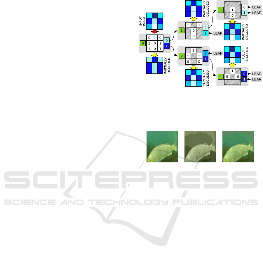
Figure 1: An example of PHIE using K=2. Each node (gray

rounded boxes) shows the ON (left), the CI (middle) and

CP (right). Dashed squares within CI denote pixels that are

not considered in that node. The images pointed by the yel-

low arrows are the partial decoding using that node and the

preceeding.

(a) (b) (c)

Figure 2: (a) Input image and the results of decoding (b)

1 node and (c) 5 nodes of the PHIE encoded image using

K=8.

that node and all of its ancestors. This error makes

it possible to sort the nodes within each tree level

depending on the amount of image information they

contain. The Order Number (ON) is computed using

this criteria and deﬁnes the speciﬁc sequence in which

the nodes have to be transmitted to guarantee that the

most part of the image information is transmitted at

the beginning.

Second, each node can be compressed. PHIE

proposes four different strategies (no compression

at all, Snappy compression, GZIP compression and

LZMA-XZ compression) ranging from faster and

larger nodes to slower and smaller nodes.

As for decoding, the entire tree can be recursively

decoded as follows. If a node is a leaf, its pixel col-

ors are picked from its own CP. Otherwise, its colors

come from decoding its child nodes. Through recur-

sion, the information will propagate from leafs up to

the root, resulting in an exact copy of the original im-

age.

Figure 1 summarizes these ideas by showing a

simple 3×3 image with 6 different colors and using

K=2. The last image, obtained from the node with an

ON of 4, is a perfect, lossless, replica of the original

one.

Combining Progressive Hierarchical Image Encoding and YOLO to Detect Fish in Their Natural Habitat

335

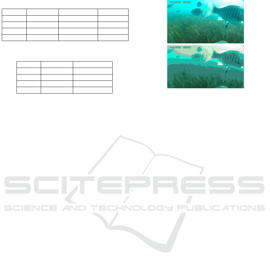
Table 1: Overview of the Luderick-Seagrass dataset.

SET # IMAGES # LUDERICK # BREAM

TRAIN 2673 6649 53

TEST 843 1632 29

VAL. 764 1023 43

TOTAL 4280 9304 125

Table 2: Overview of the processed Luderick-Seagrass

dataset.

SET # IMAGES # LUDERICK

TRAIN 2625 6416

TEST 814 1611

VAL. 721 925

TOTAL 4160 8952

As an example, we encoded the image shown in

Figure 2-a, which is part of the dataset used in the ex-

periments, using K=8 and LZMA-XZ compression.

The resulting PHIE tree has 10772 nodes. Figures 2-

b and 2-c show the result of decoding the tree using

one and ﬁve, respectively, of the 10772 nodes. As it

can be observed, only one node leads to an accept-

able quality, though still far from the original image,

whilst ﬁve nodes produce an image very similar to the

original one. The required size to store the ﬁrst ﬁve

nodes responsible for Figure 2-c is only a 31% and

a 11% of the PNG and raw versions, respectively, of

the input image. Thus, visually good images can be

obtained with a small fraction of the PHIE tree (5 of

10772 nodes) and small data size.

3 EXPERIMENTAL RESULTS

3.1 The Data

Our proposal will be evaluated using the Luderick-

Seagrass dataset (Ditria et al., 2021), which comprises

annotated footage of Girella tricuspidata in two estu-

ary systems in southeast Queensland, Australia. The

dataset contains video sequences and color images

with a resolution of 1920x1080 where two ﬁsh species

(luderick and bream) are annotated. Table 1 summa-

rizes the dataset contents.

As it can be observed, the dataset is extremely un-

balanced towards the Luderick class, with very few

instances of bream. For this reason, we removed all

the images that contained breams to have a single

class dataset. Also, we resized all the images to have

a width of 640 pixels to facilitate its use in YOLOv5.

Table 2 summarizes the resulting dataset, which is the

one used in the experiments. For the sake of clarity,

let this dataset be called the raw dataset.

Figure 3: Example of a dataset image (top) and the encoded

version (bottom).

3.2 Experimental Setup

Our goal being to experimentally evaluate the

YOLOv5 performance in detecting ﬁsh from PHIE

encoded images, we started by encoding the raw

dataset. To this end, we used K = 4, K-Means clus-

tering (KC) and Snappy compression, which lead to

good results with general purpose image quality met-

rics. Each image in the dataset was encoded up to

a size which is, approximately, the 30% of the corre-

sponding PNG encoded size in the raw dataset. In this

way, we will evaluate how good are the object detec-

tion results when only a fraction of the size needed

to encode the image in PNG is used. It is important

to emphasize that, given that PHIE nodes are atomic

(they have either to be fully transmitted or not trans-

mitted at all) it is not possible to guarantee an exact

30% of the size. More speciﬁcally, the PHIE encod-

ing we have used requires, in average, a 30.2% of the

size of PNG corresponding image with a standard de-

viation of 1.3%. Let the result of encoding each raw

dataset image using PHIE as described be referred to

as the encoded dataset. Figure 3 shows an example of

one raw dataset image together with its counterpart in

the encoded dataset.

After that, we trained three different YOLOv5

model sizes (small or YOLOv5s, medium or

YOLOv5m and large or YOLOv5l) using the train

data both from the raw dataset and from the encoded

dataset, resulting in six different conﬁgurations. Fig-

ure 4 shows the evolution of the YOLOv5 box loss

functions with the training epochs with each of the

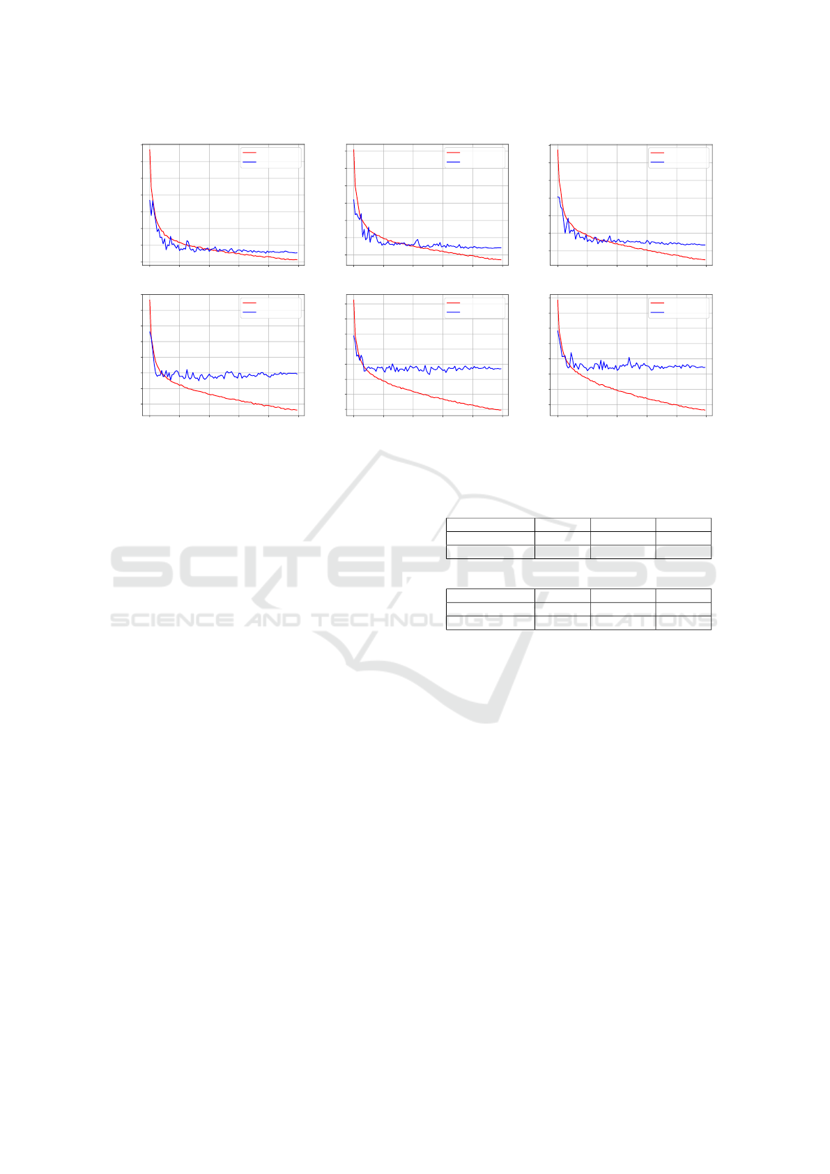
tested conﬁgurations. It can be observed how the evo-

lution is similar among model sizes. Also, it can be

observed how the models trained with the encoded

dataset start to overﬁt earlier (≃ 10 epochs) than those

trained with the raw one (≃ 30 epochs). Since it is

advisable to stop training as soon as overﬁtting ap-

VISAPP 2024 - 19th International Conference on Computer Vision Theory and Applications

336

0 20 40 60 80 100

EPOCH

0.02

0.03

0.04

0.05

0.06

0.07

0.08

0.09

BOX LOSS

INPUT DATASET, YOLOv5s

TRAINING

VALIDATION

0 20 40 60 80 100

EPOCH

0.02

0.03

0.04

0.05

0.06

0.07

0.08

BOX LOSS

INPUT DATASET, YOLOv5m

TRAINING

VALIDATION

0 20 40 60 80 100

EPOCH

0.02

0.03

0.04

0.05

0.06

0.07

0.08

BOX LOSS

INPUT DATASET, YOLOv5l

TRAINING

VALIDATION

0 20 40 60 80 100

EPOCH

0.03

0.04

0.05

0.06

0.07

0.08

0.09

0.10

BOX LOSS

ENCODED DATASET, YOLOv5s

TRAINING

VALIDATION

0 20 40 60 80 100

EPOCH

0.02

0.03

0.04

0.05

0.06

0.07

0.08

0.09

BOX LOSS

ENCODED DATASET, YOLOv5m

TRAINING

VALIDATION

0 20 40 60 80 100

EPOCH

0.02

0.03

0.04

0.05

0.06

0.07

0.08

0.09

BOX LOSS

ENCODED DATASET, YOLOv5l

TRAINING

VALIDATION

Figure 4: Evolution of the box loss with the training epochs when using the raw dataset (top row) and the encoded dataset

(bottom row) when training the small YOLO model (left column), the medium YOLO model (mid column) and the large one

(right column).

pears, this shows that using the encoded dataset leads

to shorter training times and, also, that probably train-

ing in this case would beneﬁt from a larger dataset.

There are two important parameters when evalu-

ating an object detector. On the one hand, the con-

ﬁdence threshold. This threshold is used to decide

whether a detected object is considered or discarded

depending on the speciﬁc conﬁdence score computed

by, in this case, YOLO. On the other hand, the Inter-

section over Union (IoU) threshold. The IoU mea-

sures the overlap between the detected object bound-

ing box and a ground truth bounding box as the area

of the intersection between both boxes divided by

the area of their union. The IoU threshold deﬁnes

the minimum IoU to consider that a detection and a

ground truth belong to the same object. In this way,

the IoU threshold is crucial to determine the number

of correct and incorrect object detections and compute

metrics such as Precision (P) or Recall (R).

Using one IoU threshold and several conﬁdence

thresholds, one can measure the corresponding P and

R. In this way, different Precision-Recall Curves can

be built, one for each tested IoU threshold. The area

below a Precision-Recall Curve constitutes, in single-

class object detection, the mean Average Precision

(mAP).

We will compute the mAP@0.5, which is the

mAP corresponding to an IoU threshold of 0.5; and

the mAP@0.5:0.95, which is the average of the mAP

using an IoU threshold of 0.5 up to the mAP using an

IoU threhold of 0.95 in intervals of 0.05. Both metrics

are widely used to evaluate object detectors.

Table 3: Object detection results using the raw dataset.

SMALL MEDIUM LARGE

mAP@0.5 0.931 0.928 0.926

mAP@0.5:0.95 0.752 0.765 0.768

Table 4: Object detection results using the encoded dataset.

SMALL MEDIUM LARGE

mAP@0.5 0.787 0.792 0.803

mAP@0.5:0.95 0.548 0.548 0.571

3.3 Results

After training the six mentioned models (YOLOv5s,

YOLOv5m and YOLOv5l with the raw dataset and

with the encoded dataset), we performed inference us-

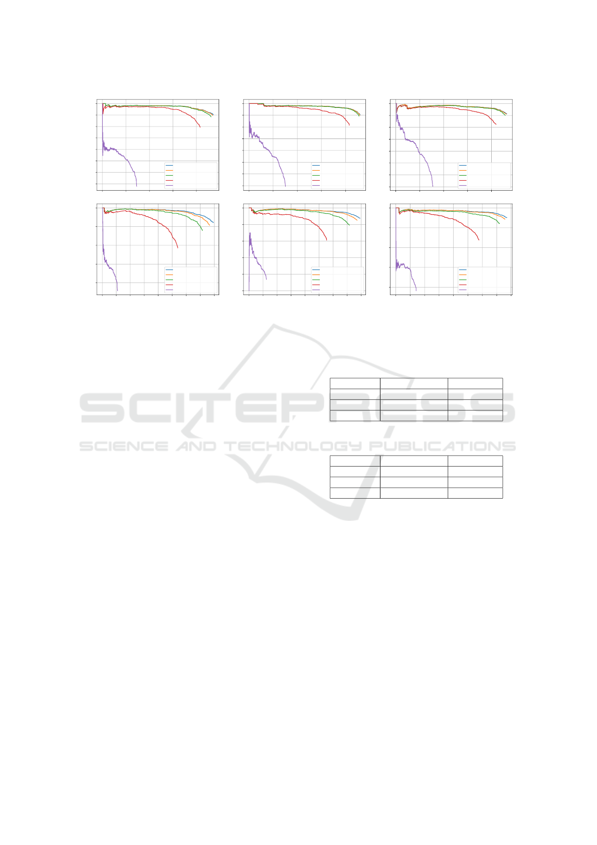
ing the test sets. Figure 5 shows the Precision-recall

curves obtained for all the six models using different

IoU thresholds. The area below each of these curves

is the corresponding mAP. It can be observed that re-

ducing the IoU threshold barely inﬂuences the results

with the raw dataset but signiﬁcant differences arise

between IoU thresholds with the encoded dataset.

Given that only small differences should appear in the

Precision-recall curves for reasonable IoU thresholds,

as it happens with the raw dataset, this reinforces the

idea that a larger trainig set would improve the results

with the encoded dataset, consistently with the results

in Figure 4.

Table 3 shows the mAP@0.5 and mAP@0.5:0.95

when using the raw dataset and Table 4 shows the

same metrics when the encoded dataset is used. Re-

sults using the raw dataset show very large mAP@0.5

Combining Progressive Hierarchical Image Encoding and YOLO to Detect Fish in Their Natural Habitat

337

0.0 0.2 0.4 0.6 0.8

Recall

0.3

0.4

0.5

0.6

0.7

0.8

0.9

1.0

Precision

IoU>=0.100, AP=0.943

IoU>=0.300, AP=0.939

IoU>=0.500, AP=0.931

IoU>=0.700, AP=0.857

IoU>=0.900, AP=0.257

0.0 0.2 0.4 0.6 0.8

Recall

0.3

0.4

0.5

0.6

0.7

0.8

0.9

1.0

Precision

IoU>=0.100, AP=0.935

IoU>=0.300, AP=0.933

IoU>=0.500, AP=0.928

IoU>=0.700, AP=0.862

IoU>=0.900, AP=0.285

0.0 0.2 0.4 0.6 0.8

Recall

0.3

0.4

0.5

0.6

0.7

0.8

0.9

1.0

Precision

IoU>=0.100, AP=0.935

IoU>=0.300, AP=0.933

IoU>=0.500, AP=0.926

IoU>=0.700, AP=0.863

IoU>=0.900, AP=0.305

0.0 0.1 0.2 0.3 0.4 0.5 0.6 0.7 0.8

Recall

0.2

0.4

0.6

0.8

1.0

Precision

IoU>=0.100, AP=0.852

IoU>=0.300, AP=0.832

IoU>=0.500, AP=0.787

IoU>=0.700, AP=0.611

IoU>=0.900, AP=0.094

0.0 0.1 0.2 0.3 0.4 0.5 0.6 0.7 0.8

Recall

0.0

0.2

0.4

0.6

0.8

1.0

Precision

IoU>=0.100, AP=0.856

IoU>=0.300, AP=0.840

IoU>=0.500, AP=0.792

IoU>=0.700, AP=0.625

IoU>=0.900, AP=0.105

0.0 0.1 0.2 0.3 0.4 0.5 0.6 0.7 0.8

Recall

0.2

0.4

0.6

0.8

1.0

Precision

IoU>=0.100, AP=0.848

IoU>=0.300, AP=0.838

IoU>=0.500, AP=0.803

IoU>=0.700, AP=0.662

IoU>=0.900, AP=0.125

Figure 5: Precision-recall curves using different IoU thresholds corresponding to YOLO trained with the raw dataset (top

row) and the encoded dataset (bottom row). The left column shows the results for YOLOv5s, the mid column corresponds to

YOLOv5m and the right column to YOLOv5l.

(greater than 0.9) and mAP@0.5:0.95 (greater than

0.7). They also show that, even though the

mAP@0.5:0.95 slightly increase with the model size,

the mAP@0.5 decreases. These changes being very

small, they are likely to be noise and, so, we can con-

clude that the model size barely inﬂuences the results

with the raw dataset.

As for the encoded dataset, the mAP@0.5 re-

sults are also good, though clearly below those ob-

tained with the raw dataset. Whereas the raw dataset

leads to mAP@0.5 larger than 0.9 in all cases, the

use of the encoded dataset reduces that metric to

values close to 0.8. A similar pattern is observed

with mAP@0.5:0.95, which exhibits values between

0.5 and 0.6 whereas the raw dataset provided values

larger than 0.7. Nevertheless, taking into account that

the image size used in the encoded dataset is less than

one third of that of the raw dataset, the small loss in

mAP is more than acceptable.

Another difference between the use of the raw and

the encoded dataset is the evolution of the results with

the model size. In the case of the encoded dataset,

the evolution is more clear, with all metrics increas-

ing with the model size. This suggests that object de-

tection with PHIE images could beneﬁt from larger

models.

Even though the Precision-recall curves and mAP

provide a meaningful insight of the overall perfor-

mance, deploying a trained model requires one spe-

ciﬁc conﬁdence threshold. To ﬁnd it, we explored the

conﬁguration space using conﬁdence thresholds rang-

ing from 0.05 to 0.95 in intervals of 0.05. For each

Table 5: Optimal conﬁdence thresholds with the raw

dataset.

THRESHOLD F1-SCORE

SMALL 0.3 0.906

MEDIUM 0.35 0.908

LARGE 0.45 0.929

Table 6: Optimal conﬁdence thresholds with the encoded

dataset.

THRESHOLD F1-SCORE

SMALL 0.5 0.754

MEDIUM 0.45 0.757

LARGE 0.35 0.776

conﬁdence threshold, we computed the F1-Score met-

ric using an IoU threshold of 0.5. The F1-Score is a

suitable metric for object detection as it balances pre-

cision and recall, effectively capturing both the abil-

ity to accurately identify objects and minimize false

positives. Then, we selected the conﬁdence threshold

maximizing the F1-Score.

Tables 5 and 6 show the conﬁdence thresholds

maximizing the F1-Score as well as the maximum

F1-Scores for the raw and the encoded datasets re-

spectively. As it can be observed, in both cases,

the larger the model the better the optimal F1-Score.

However, the optimal conﬁdence threshold increases

with the model size when the raw dataset is used

whilst it decreases when using the encoded one. Since

longer training will consolidate the conﬁdence thresh-

old around that using to compute the loss function

during training (0.5), this is consistent with previous

results, suggesting that there is still room to train the

VISAPP 2024 - 19th International Conference on Computer Vision Theory and Applications

338

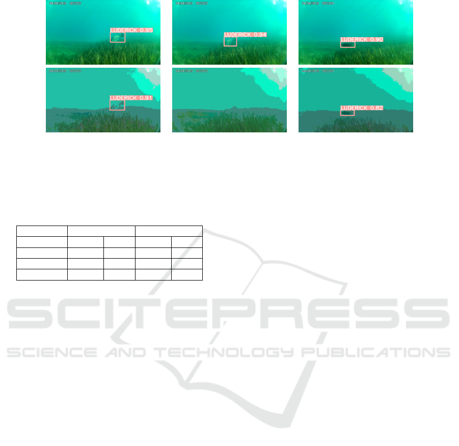
Figure 6: An instance of failure with the encoded dataset. Top row: detections on the raw dataset. Bottom row: corresponding

detections on the encoded dataset. The text near the bounding box states the class (luderick) and the conﬁdence score assigned

by YOLO.

Table 7: Mean (µ) and standard deviation (σ) of the in-

ference times per image expressed in ms for all the tested

model sizes and datasets.

RAW ENCODED

µ σ µ σ

SMALL 9.505 0.693 8.601 0.789

MEDIUM 18.938 0.628 19.353 0.620

LARGE 39.307 0.467 40.127 0.581

model with larger encoded datasets.

By carefully checking the detection on the en-

coded images sorted by the video frame from which

they come from, we have observed that the instances

of failure tend to be spurious errors (positives or neg-

atives), spending one or two frames. Figure 6 exem-

pliﬁes this idea. In this example, the ﬁsh is detected in

all frames with the raw dataset, but the mid frame is

lost in the encoded dataset. This is a key feature since

these failures can be easily corrected by considering

the temporal continuity of the input video sequence

by, for example, performing ﬁsh tracking.

Finally, we measured the detection times in each

of the images for all the tested datasets and model

sizes. The times have been measured on a standard

laptop (i7 CPU at 2.60GHz with 16 GB RAM running

Ubuntu 20.04) endowed with a NVIDIA GeForce

GTX 1650 with 4 GB and executing YOLOv5 on

Python-3.8.10 with torch-1.11.0 and CUDA 11.3.

The mean and the standard deviation of the detec-

tion times are reported in Table 7. As it can be ob-

served, each model approximately duplicates the in-

ference time of the immediately smaller one. Also,

there are no signiﬁcant differences between the raw

and the encoded dataset, both of them being suitable

for video-rate processing in most cases.

4 CONCLUSION

In this paper we have experimentally evaluated the

performance of YOLOv5 to detect ﬁsh in underwa-

ter images when partially decoded PHIE images are

used. This makes it possible to evaluate the feasibil-

ity of using PHIE for underwater image transmission

when the intended task is to perform ﬁsh detection.

The experimental setup considered both the orig-

inal images (raw dataset) and the partially decoded

ones up to a 30% of the original image size in PNG

format (encoded dataset). In other words, the partial

decoding will use only a 30% of the bandwidth re-

quired by the corresponding PNG image, making it

possible for an AUV to transmit the images fastly to

a, for example, base station in charge of performing

ﬁsh detection.

As for ﬁsh detection, we used YOLOv5 and

tested three different model sizes: the small one

(YOLOv5s), the medium one (YOLOv5m) and the

large one (YOLOv5l).

Results show smaller performance when using the

encoded dataset. Whereas the mAP@0.5 surpasses

the 0.9 with the raw data, it barely reaches the 0.8

when using the encoded dataset. However, two as-

pects favour the use of PHIE. On the one hand, it is a

small performance reduction considering the substan-

tial gain in image size. On the other hand, an in-depth

analysis of the intances of failure shows that errors

are, in general, spurious, involving only one or two

frames of the original video sequence. This kind of

errors can be easily detected and, even, corrected by

considering the temporal sequence when, for exam-

ple, performing ﬁsh tracking or counting.

Overall, using PHIE seems to be a good option

when performing ﬁsh detection if the communication

bandwidth or reliability is more important than the

overall detection rate.

Combining Progressive Hierarchical Image Encoding and YOLO to Detect Fish in Their Natural Habitat

339

Future work involves studying the behavior of

YOLOv5 using different partial decodings, not only

using a 30% of the PNG size but exploring a larger

range. Also, even though YOLOv5 is mature and

widely spread, testing more recent YOLO versions

could provide additional insight into the advantages

of performing ﬁsh detection using partially decoded

data.

Finally, we would like to emphasize that we have

made all the source code used in this paper publicly

available. The PHIE is available at https://github.com/

aburguera/PHCENCODER. A YOLOv5 wrapper as

well as different tools to compute different metrics

and perform grid search on different parameters is

available at https://github.com/aburguera/ODUTILS.

ACKNOWLEDGEMENTS

This work is partially supported by

Grant PID2020-115332RB-C33 funded by

MCIN/AEI/10.13039/501100011033 by ”ERDF

A way of making Europe” and by Grant PLEC2021-

007525/AEI/10.13039/501100011033 funded by the

Agencia Estatal de Investigacion, under NextGenera-

tion EU/PRTR

REFERENCES

Anwar, S. and Li, C. (2020). Diving deeper into underwa-

ter image enhancement: A survey. Signal Processing:

Image Communication, 89:115978.

Bonin-Font, F. and Burguera, A. (2020). Towards multi-

robot visual graph-SLAM for autonomous marine ve-

hicles. Journal of Marine Science and Engineering,

8(6).

Burguera, A. (2023). Hierarchical color encoding for

progressive image transmission in underwater envi-

ronments. IEEE Robotics and Automation Letters,

8(5):2970–2975.

Burguera, A. and Bonin-Font, F. (2022). Progressive hierar-

chical encoding for image transmission in underwater

environments. In OCEANS 2022 - Hampton Roads,

pages 1–9.

Burguera, A., Bonin-Font, F., Lisani, J. L., Petro, A. B.,

and Oliver, G. (2016). Towards automatic visual sea

grass detection in underwater areas of ecological in-

terest. In 2016 IEEE 21st International Conference

on Emerging Technologies and Factory Automation

(ETFA), pages 1–4.

Ditria, E. M., Connolly, R. M., Jinks, E. L., and Lopez-

Marcano, S. (2021). Annotated video footage for au-

tomated identiﬁcation and counting of ﬁsh in uncon-

strained seagrass habitats. Frontiers in Marine Sci-

ence, 8.

Do, H., Hong, S., and Kim, J. (2020). Robust Loop Closure

Method for Multi-Robot Map Fusion by Integration of

Consistency and Data Similarity. IEEE Robotics and

Automation Letters, 5(4):5701–5708.

Feng, W., Hu, C., Wang, Y., Zhang, J., and Yan, H. (2019).

A novel hierarchical coding progressive transmission

method for wmsn wildlife images. Sensors, 19(4).

Guo, J.-M. (2010). High efﬁciency ordered dither block

truncation coding with dither array lut and its scal-

able coding application. Digital Signal Processing,

20(1):97–110.

He, K., Gkioxari, G., Doll

ar, P., and Girshick, R. (2017).

Mask R-CNN.

Jaafar, A. N., Ja’afar, H., Pasya, I., Abdullah, R., and Ya-

mada, Y. (2022). Overview of underwater commu-

nication technology. In Proceedings of the 12th Na-

tional Technical Seminar on Unmanned System Tech-

nology 2020, pages 93–104, Singapore. Springer Sin-

gapore.

oser, K. and Frese, U. (2020). Challenges in Underwater

Visual Navigation and SLAM. In Intelligent Systems,

Control and Automation: Science and Engineering,

volume 96, pages 125–135.

Latif, Y., Cadena, C., and Neira, J. (2013). Robust loop

closing over time for pose graph SLAM. International

Journal of Robotics Research, 32(14):1611–1626.

Lin, T.-Y., Goyal, P., Girshick, R., He, K., and Doll

ar, P.

(2020). Focal loss for dense object detection. IEEE

Transactions on Pattern Analysis and Machine Intel-

ligence, 42(2):318–327.

Monika, R., Samiappan, D., and Kumar, R. (2021). Under-

water image compression using energy based adaptive

block compressive sensing for IoUT applications. The

Visual Computer, (37):1499–1515.

Redmon, J., Divvala, S., Girshick, R., and Farhadi, A.

(2016). You only look once: Uniﬁed, real-time ob-

ject detection. In 2016 IEEE Conference on Com-

puter Vision and Pattern Recognition (CVPR), pages

779–788, Los Alamitos, CA, USA. IEEE Computer

Society.

Rubino, E. M., Centelles, D., Sales, J., Marti, J. V., Marin,

R., Sanz, P. J., and Alvares, A. J. (2017). Progressive

image compression and transmission with region of

interest in underwater robotics. In OCEANS 2017 -

Aberdeen, pages 1–9.

Said, A. and Pearlman, W. (1996). A new, fast, and efﬁcient

image codec based on set partitioning in hierarchical

trees. IEEE Transactions on Circuits and Systems for

Video Technology, 6(3):243–250.

Tan, M., Pang, R., and Le, Q. V. (2020). EfﬁcientDet: Scal-

able and efﬁcient object detection. In 2020 IEEE/CVF

Conference on Computer Vision and Pattern Recogni-

tion (CVPR), pages 10778–10787.

Ultralytics. YOLOv5.

https://github.com/ultralytics/yolov5. Accessed:

2023-11-14.

Viola, P. and Jones, M. (2001). Rapid object detection us-

ing a boosted cascade of simple features. In Proceed-

ings of the 2001 IEEE Computer Society Conference

on Computer Vision and Pattern Recognition. CVPR

2001, volume 1, pages I–I.

VISAPP 2024 - 19th International Conference on Computer Vision Theory and Applications

340