Deep Learning Model Compression for Resource Efﬁcient Activity

Recognition on Edge Devices: A Case Study

Dieter Balemans

1,3

, Benjamin Vandersmissen

, Jan Steckel

, Siegfried Mercelis

, Phil Reiter

and Jos

e Oramas

Faculty of Applied Engineering, University of Antwerp - imec - IDLab, Sint-Pietersvliet 7, 2000 Antwerp, Belgium

Faculty of Science, University of Antwerp - imec - IDLab, Sint-Pietersvliet 7, 2000 Antwerp, Belgium

Faculty of Applied Engineering, University of Antwerp - CoSysLab, Groenenborgerlaan 171, 2020 Antwerp, Belgium

Keywords:

Activity Recognition, Model Compression, Pruning, Quantization, Edge Computing.

Abstract:

This paper presents an approach to adapt an existing activity recognition model for efﬁcient deployment on

edge devices. The used model, called YOWO (You Only Watch Once), is a prominent deep learning model.

Given its computational complexity, direct deployment on resource-constrained edge devices is challenging.

To address this, we propose a two-stage compression methodology consisting of structured channel pruning

and quantization. The goal is to signiﬁcantly reduce the model’s size and computational needs while main-

taining acceptable task performance. Our experimental results, obtained by deploying the compressed model

on Raspberry Pi 4 Model B, conﬁrm that our approach effectively reduces the model’s size and operations

while maintaining satisfactory performance. This study paves the way for efﬁcient activity recognition on

edge devices.

1 INTRODUCTION

Activity recognition is a crucial task in various in-

dustries, including unmanned aerial vehicle monitor-

ing, autonomous driving, and urban security systems.

However, one of the challenges in this ﬁeld is the

computational complexity associated with large deep

learning models. This, makes it infeasible to deploy

these models on edge devices, where resources are

generally limited. Nevertheless, the recent push to-

ward making decisions at the edge extends to the ﬁeld

of activity recognition. For example, activity recogni-

tion is being used on remote construction sites for on-

site progress monitoring (IMEC, 2023)(Braun et al.,

2020). Deploying complex algorithms on edge de-

vices offers several beneﬁts. Firstly, it reduces sys-

tem latency since data does not need to be sent to the

cloud for processing. This also enhances the security

and privacy of the system as data does not leave the

device. Lastly, it decreases the cost of the system, as it

removes the need for a powerful server to process the

data. Therefore, we aim to investigate the feasibility

of deploying deep learning-based activity recognition

on edge devices. More speciﬁcally, we will explore

how to adapt existing deep learning models to make

them suitable for edge deployment.

This paper focuses on the YOWO (You Only

Watch Once) model proposed by K

ukl

u et

al. (K

ukl

u et al., 2019). YOWO is a widely used

convolutional neural network architecture for activity

recognition. However, due to its size and complexity,

it is not initially suitable for edge deployment. The

goal is to adapt this model an make it more suitable

for edge computing, by reducing its size and opera-

tions. The target device is the Raspberry Pi 4 Model

B. We aim for the model to maintain high enough per-

formance while ﬁtting within an applications require-

ments. These requirements can be a time (latency)

constraint, a memory constraint or an energy con-

straint. To achieve this, we propose a two-stage com-

pression approach: structured channel pruning and

quantization.

In the ﬁrst stage, structured channel pruning, our

goal is to decrease the size of the model and the num-

ber of operations needed to execute the model, with-

out affecting its accuracy. This technique selectively

removes channels from convolutional layers, result-

ing in a smaller and faster model. This is because ten-

sors can be reduced in size without the need for spe-

cialized hardware. Moreover, we merge pruning with

quantization to further shrink the model’s size by rep-

resenting the weights and activations with fewer bits.

Balemans, D., Vandersmissen, B., Steckel, J., Mercelis, S., Reiter, P. and Oramas, J.

Deep Learning Model Compression for Resource Efﬁcient Activity Recognition on Edge Devices: A Case Study.

DOI: 10.5220/0012423300003660

Paper published under CC license (CC BY-NC-ND 4.0)

In Proceedings of the 19th International Joint Conference on Computer Vision, Imaging and Computer Graphics Theory and Applications (VISIGRAPP 2024) - Volume 4: VISAPP, pages

575-584

ISBN: 978-989-758-679-8; ISSN: 2184-4321

575

We present our compression approach in combi-

nation with a sensitivity analysis to determine the im-

pact of pruning the model and to ﬁnd the optimal pa-

rameters for scheduling the pruning. We assess the

effectiveness of our approach by deploying the com-

pressed YOWO model on the Raspberry Pi 4 Model

B. We then measure its latency, energy consumption,

and memory usage. The results show that we can con-

siderably decrease the latency and memory consump-

tion of the YOWO model while keeping task perfor-

mance at an acceptable level.

In the next section we provide an overview of

related work in the ﬁeld of activity recognition and

deep learning model compression. Section 3.1 de-

scribes the YOWO model and its training process.

Sections 3.2 and 3.3 explain the compression tech-

niques used in this work. Section 4 describes the

experimental setup and presents the results. Finally,

Section 5 concludes the paper and discusses future

work.

2 RELATED WORK

Activity Recognition. Activity recognition is the task

of recognizing activities from a sequence of frames.

In other words, it is the spatiotemporal localization

of activities in observations. Numerous approaches

have been proposed to solve this task. A common ap-

proach is to use a sliding window to extract features

from the observations and use these features to clas-

sify the activity. The features can be extracted using

a variety of methods, such as hand-crafted features,

or deep learning. Earlier deep learning methods, rely

on a two-stream convolutional neural network (CNN)

to extract spatial and temporal features separately and

fuse them to classify the activity (Simonyan and Zis-

serman, 2014)(Feichtenhofer et al., 2016). However,

these methods are computationally expensive and can

be very time-consuming. More recently, the use of

3D CNNs has become more popular. Its is able to

learn both spatial and temporal features simultane-

ously. These models are proven to perform better on

the activity recognition task (Qiu et al., 2017)(Tran

et al., 2017)(Feichtenhofer et al., 2018)(Tran et al.,

2014). However, these models are even more expen-

sive in terms of size and operations. 3D convolutions

have much more parameters and require more opera-

tions than 2D convolutions. This makes them difﬁcult

to deploy on edge devices. Therefore, in this work,

we investigate the possibility of compressing a 3D

CNN for activity recognition. We choose the YOWO

model proposed by K

ukl

u et al. (K

ukl

u et al.,

2019) as base model. This model is a uniﬁed, single-

stage architecture which consist of 2 two branches.

The YOWO model is the fastest model for activity

recognition, however, it is still too large for edge de-

ployment. We provide more details about the model

in Section 3.1.

Compression. Neural network compression is a ﬁeld

of research that aims to reduce the size and operations

of a neural network. There are several techniques that

can be used to achieve this. Techniques like pruning

and quantization are among the most popular ones,

and often used in combination. Pruning is the pro-

cess of removing weights, neurons or channels from a

neural network. In the ﬁeld there are numerous tech-

niques, all which differ in the way to determine the

importance of connections (i.e. where to remove con-

nections), the granularity (i.e. which connections to

remove) and the scheduling (i.e. when to remove con-

nections). Generally, pruning is done by removing the

connections and neurons that have the smallest im-

pact on the network’s output. This paved the way to

pruning methods based on weights (Han et al., 2016),

activations (Georgiadis, 2018) and gradients (Liu and

Wu, 2019). For instance, Lee et al. (Lee et al., 2018)

use a saliency-based criterion consisting of the lowest

absolute value of the normalized gradient multiplied

by the weight magnitude for a given set of mini-batch

inputs.

For the granularity, there are two main types

of pruning: unstructured (Frankle and Carbin,

2018)(Tanaka et al., 2020) and structured pruning (Li

et al., 2016)(He et al., 2017). Unstructured prun-

ing removes individual connections from the network.

This means the weight tensor of the network will be

very sparse and highly irregular. These methods allow

for the highest compression rates with the lowest im-

pact on accuracy. However, this sparsity is (currently)

not suitable for hardware acceleration. On the other

hand, structured pruning removes entire block-like

structures from the network (Crowley et al., 2018).

For example, in channel pruning, entire channels of a

convolutional layer are removed. This allows for the

weight tensors to be actually smaller by removing the

entire row or column of the channel, removing a lot

of OPs (operations). On current hardware, and espe-

cially on CPU only devices, this is the most suitable

type of pruning. One drawback of structured pruning

is that it is less ﬂexible than unstructured pruning, and

has a much bigger impact on the network’s perfor-

mance. In this work we focus on structured pruning,

more speciﬁcally channel pruning.

In this work we combine pruning with quantiza-

tion. We follow the philosophy of the work of Han

et al. (Han et al., 2016) where pruning is combined

with quantization. They show that quantizing after

VISAPP 2024 - 19th International Conference on Computer Vision Theory and Applications

576

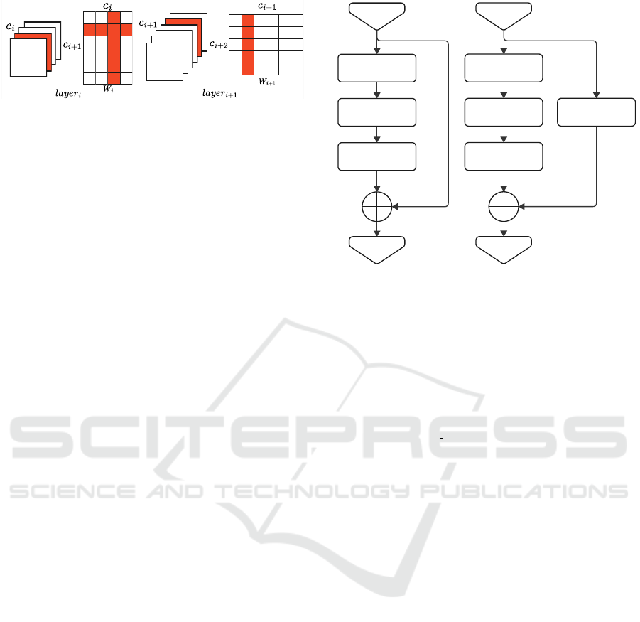
Figure 1: Overview of the structured channel pruning pro-

cess. Here we show the removal of one channel from layer i

and one channel from layer i + 1. The effect of the removal

is visible in red.

pruning is possible without losing accuracy. There-

fore, we propose a similar approach in this work for

compression of large activity recognition models.

3 METHODOLOGY

3.1 Activity Recognition

As mentioned previously, we use the You Only Watch

Once (YOWO) model (K

ukl

u et al., 2019) as our

baseline model. YOWO is a single-stage architecture

which consist of 2 two branches to extract temporal

and spatial information from video frames. Speciﬁ-

cally, the 2D backbone is a YoloV2 model (Darknet-

19) (Redmon and Farhadi, 2016). The 3D backbone

is a ResNext-101 model (Xie et al., 2016). Ultimately,

the model predicts the activity class and the bounding

box of the activity in the video frame. Note that there

are variation of the YOWO model with different 2D

and 3D backbone conﬁgurations. For this paper we

only use the standard (Darknet-19 and ResNext-101)

conﬁguration. The goal is the evaluate the compres-

sion of this standard conﬁguration.

This conﬁguration makes the model altogether a

fairly large model, with over 121 million parame-

ters and 43 billion operations, making it difﬁcult for

deployment on edge devices with limited resources.

Therefore, we investigate the possibility of compress-

ing the YOWO model to enable inference and analysis

on the edge device. In the next section we will discuss

the compression techniques that we use to compress

the model.

In this work we perform post-training compres-

sion. This means we train the YOWO model before-

hand, and use it as a starting point for the compression

process. We provide more details about the training

and evaluation in section 4.

3.2 Neural Network Pruning

In this work we employ neural network pruning to re-

duce the size and amount of operations of the YOWO

conv1: 3x3, 128

conv2: 1x1, 64

conv3: 3x3, 128

input

128- d

output

128- d

conv1: 3x3, 128

conv2: 1x1, 64

conv3: 3x3, 128

input

256- d

output

128- d

conv_down: 3x3, 128

Figure 2: Sample of bottleneck blocks as used in the YOWO

model. (Left) An example of a bottleneck block with-

out downsampling layer. The block takes in 128 channels.

In this block, the addition operation creates a dependency

between the channels of the third convolution operation

(conv3: 3x3, 128), the ﬁrst convcolution operation (conv1:

1x1, 128) and the input. (Right) An example of a bottle-

neck block with downsampling layer. The block takes in

256 channels. In this block, the addition operation creates a

dependency between the channels of the third convolution

operation (conv3: 3x3, 128), the downsampling convolu-

tion operation (conv down: 3x3, 128), the ﬁst convcolution

operation (conv1: 1x1, 128) and the input.

model. We use a structured iterative channel prun-

ing technique (Wen et al., 2016) to remove unim-

portant channels from the convolutional layers of the

YOWO model. The YOWO model has both 2D and

3D convolutional layers. In both cases we use the

same pruning technique. In order to estimate the im-

portance of each channel, we use two different cri-

teria: weight magnitude (Han et al., 2016) and ac-

tivation (Georgiadis, 2018). The weight magnitude

criterion is based on the magnitude of the connection

weights. We utilize the l

-norm of the weights to de-

termine the importance of each channel. The activa-

tion criterion is based on the activation of the neu-

rons. We follow the same approach to estimate the

importance of each channel, using the l

-norm, but

this time using the output activations instead of the

weights. We compare the results of both criteria in

Section 4.

The pruning process itself is scheduled in an itera-

tive fashion. In each iteration, we prune a certain per-

centage of the channels from the layers. This is fol-

lowed by a ﬁne-tuning step, where we ﬁne-tune the

model to recover the performance lost during prun-

ing. As we will see in our sensitivity analysis re-

sults in Section 4, the pruning process can be quite

Deep Learning Model Compression for Resource Efﬁcient Activity Recognition on Edge Devices: A Case Study

577

Train Model

Prune

Model

Model Pruning

Importance

Calculation

Channel

masking

Fine Tuning

Quantize Model

(optional)

Quantization

Fuse Layers

Calibration

using test data

Static

Quantization

Export to

ONNX

Deploy

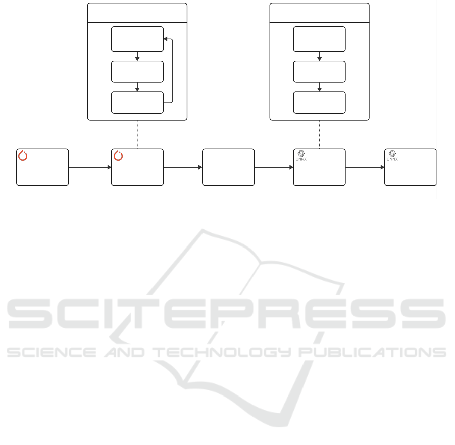
Figure 3: Overview of the full compression pipeline. The pipeline starts with training the model in PyTorch. Then we prune

the model using structured channel pruning. After pruning, we export the model to the ONNX format. Next, we quantize the

model using static post-training quantization. Finally, the model can be deployed on the target device.

aggressive. Especially when pruning both the 2D and

3D backbone simultaneously. Therefore, we split the

pruning process into two phases. In the ﬁrst phase,

we prune the 2D backbone and ﬁne-tune the model.

In the second phase, we prune the 3D backbone and

ﬁne-tune the model. This way, we can have ﬁner con-

trol of the pruning and prevent the performance drop

from becoming unrecoverable.

As explained before, we opted for a structured

pruning technique, as opposed to unstructured prun-

ing. This because structured pruning is more suitable

for deployment on edge devices. Unstructured prun-

ing techniques, such as magnitude-based pruning as

used in the Lottery Ticket Hypothesis (Frankle and

Carbin, 2018), are very effective in creating sparse

models that maintain performance very well. How-

ever, since the tensors are sparse in a very irregular

fashion, it is difﬁcult to take advantage of this sparsity

in the inference phase. Therefore, we use structured

pruning techniques, such as channel pruning, which

create sparse models in a structured fashion. This

structure allows us to take advantage of the sparsity

in the inference phase. Using channel pruning we can

remove entire channels from the convolutional layers,

resulting in physically smaller tensors. This is shown

in Figure 1. This results in smaller models, that re-

quire less operation and gain a speedup natively from

the sparsity. It is important to note that due to the

models architecture, not all channels can be pruned.

We have to make sure the model matrix operations re-

main valid. For example, this is the case when we use

bottleneck blocks (shown in Figure 2) where the num-

ber of input channels needs to be equal to the number

of output channels, since we add the input to the out-

put. These dependencies between channels are taken

into account when pruning the model.

3.3 Quantization

We use quantization to further reduce the size of the

YOWO model. Quantization involves representing

the weights and/or activation with fewer bits. The

original model uses 32-bit ﬂoating point numbers to

represent the weights and activations. In this work

we use static post-training quantization (PTQ) (Kr-

ishnamoorthi, 2018). We quantize the model after

training and pruning. This method is static because

the quantization parameters are calculated once and

are ﬁxed. The goal is that after quantization both the

weights and activations are represented with 8-bit in-

tegers. This allows for a signiﬁcant reduction in size

for storing the model, and depending on hardware and

software support, a reduction in latency as well.

This process is performed in two steps. The ﬁrst

step is a calibration step where we collect statistics

of the weights and activations. In our case we collect

the minimum and maximum values of the weights and

activations. These values are subsequently used for a

range-based linear quantization (Jacob et al., 2017).

This is done by running the model on a representative

test dataset. The second step is the actual quantization

step. Here the actual weights and model operations

are replaced with the quantized counterparts.

It is important to note that after quantization

various hardware and software limitations arise.

We perform the quantization in the ONNX frame-

work (ONNX, 2023). This makes deployment of the

compressed model easier, since the ONNX frame-

VISAPP 2024 - 19th International Conference on Computer Vision Theory and Applications

578

work is supported by many platforms, including the

Raspberry Pi 4 Model B. However, currently, the

ONNX framework (and its execution providers) does

not support all operation types in quantized form on

our target device. This means that, though the mod-

els weights are quantized, the operations are still per-

formed in ﬂoating point depending on hardware sup-

port. This means the main beneﬁt of quantization in

this work is storage, not latency.

3.4 Full Compression Pipeline

In this section, we provide an overview of the full

compression pipeline. In Figure 3, we show the com-

plete pipeline. We begin with the original YOWO

model trained in PyTorch. Then, we prune the model

using the structured channel pruning technique de-

scribed in Section 3.2. After pruning, the model is

exported to the ONNX format. Next, we quantize the

model using the post-training quantization technique

described in Section 3.3. As mentioned the main ben-

eﬁt of quantization is storage reduction, not latency

improvement. Therefore, this quantization step is op-

tional if the model is already small enough. Finally,

the model can be deployed on the target device, which

in our case is the Raspberry Pi 4 Model B. We utilize

the ONNX runtime for inference of the model on the

device. Once all of these steps are completed, we can

measure the latency, energy consumption, and mem-

ory usage of the model on the device. The results of

these measurements are presented in Section 4.3.

4 EXPERIMENTS AND RESULTS

In this section we describe the experiments we per-

formed to evaluate the performance of the proposed

compression pipeline. The experiments involve using

the originally trained activity recognition model as

described in Section 3.1. The compression is, just as

the performance evaluation, task dependent. There-

fore, before we propose an actual pruning schedule

for the full compression stack, we perform a sensi-

tivity analysis on the model. A sensitivity analysis

is a common technique used to determine the impact

of pruning the model, and allows us to ﬁnd the opti-

mal parameters for scheduling the pruning. In this pa-

per we perform experiments using the YOWO model

trained on two different datasets. The JHMDB-21

dataset (Jhuang et al., 2013) is a subset of the HMDB-

51 dataset (Kuehne et al., 2011) and contains 928

short videos of 21 different activities. Each video has

a single action across all frames. The actions in this

dataset include human actions and poses. The UCF-

24 dataset is a subset of the UCF-101 dataset (Soomro

et al., 2012) and contains 3207 videos of 24 differ-

ent activities. In this dataset multiple instances of the

same activity can occur in a single video. The actions

in this dataset are more related to sports activities.

The YOWO model is trained on both datasets sepa-

rately and each model is used as a starting point for

the compression process. The models are trained us-

ing standard gradient descent with the AdamW opti-

mizer (Loshchilov and Hutter, 2017). More informa-

tion about the training of these baseline models, such

as the used hyperparameters, can be found in Sec. 5.

The compression itself was computed on a Nvidia

Tesla V100-SXM2-32GB GPU. The resource con-

sumption was measured on a Raspberry Pi 4 Model B.

We assess model compression in two ways: by eval-

uating resource consumption and task performance.

For the resource consumption, we focus on the com-

putational complexity and measurements on a target

device. This is done by measuring a range of met-

rics, including: (i) the number of parameters, (ii) the

number of operations (FLOPs or OPs), (iii) the model

ﬁle size (quantized and unquantized), (iv) the models

compression ratio ((Eq. I)

size

original

size

compressed

), (v) the mod-

els theoretical speedup ((Eq. II)

#OPs

original

#OPs

compressed

), (vi) the

models latency measured on a target device, (vii) the

models runtime memory usage measured on a tar-

get device, (viii) and the models energy consumption

measured on a target device. The task performance is

evaluated by measuring the performance of the model

on the on a validation dataset. For this we use the

mean Average Precision (mAP) metric. More speciﬁ-

cally we use the frame-mAP metric. This metric mea-

sures the area under the precision-recall curve of de-

tection for each frame. The mAP is calculated using

a IoU threshold of 0.5.

In the next section, we show the results for the

performed sensitivity analysis on the YOWO model.

Afterwards, we use the results of this analysis to

set up a pruning schedule for the full compression

pipeline. We show results of the full compression

pipeline using multiple different schedules. Finally, in

section 4.3 results of the resource consumption mea-

surements on the Raspberry Pi 4 Model B are shown.

4.1 Sensitivity Analysis

As mentioned, we utilize a sensitivity analysis to

make an informed decision regarding the pruning cri-

terion to be employed in the full compression stack.

This analysis entails pruning the network using a spe-

ciﬁc criterion and measuring its performance as the

level of sparsity increases. The objective is to deter-

Deep Learning Model Compression for Resource Efﬁcient Activity Recognition on Edge Devices: A Case Study

579

Table 1: Results of the full compression pipeline (pruning and quantization). The models are labeled using an ID. This ID

is used in the following tables to refer to the models. Results are shown for the JHMDB-21 and UCF-24 datasets. The mAP

and Q. mAP are the mean average precision of the original and quantized models, respectively. The Params and OPs are

the number of parameters and operations of the models. The Size and Q. Size are the size of the compressed and quantized

models. The Speedup is the calculated theoretical speedup (Eq. II) of the compressed model compared to the original model.

ID Dataset Attribution mAP / Q. mAP (%) Params OPs Size / Q. Size (MB) Speedup

0 JHMDB-21 — 67.54 / 66.76 1.21e+08 4.34e+10 462.00 / 121.61 1.00

1 JHMDB-21 weight 62.77 / 62.08 7.02e+07 2.06e+10 282.45 / 70.90 2.10

2 JHMDB-21 weight 56.66 / 55.30 6.74e+07 1.59e+10 271.04 / 68.05 2.73

3 JHMDB-21 activation 71.51 / 71.10 7.02e+07 3.54e+10 282.25 / 70.86 1.23

4 JHMDB-21 activation 60.69 / 59.07 6.88e+07 1.87e+10 276.66 / 69.46 2.32

5 JHMDB-21 activation 32.23 / 32.17 5.95e+07 1.37e+10 239.30 / 60.12 3.16

6 UCF-24 — 75.87 / 75.80 1.21e+08 4.34e+10 462.00 / 121.63 1.00

7 UCF-24 weight 75.61 / 75.53 1.01e+08 1.05e+10 404.07 / 101.30 4.15

8 UCF-24 weight 73.63 / 72.03 8.31e+07 9.09e+09 333.56 / 83.68 4.78

9 UCF-24 activation 75.85 / 73.43 8.48e+07 7.73e+09 340.39 / 85.38 5.62

10 UCF-24 activation 71.94 / 71.43 6.83e+07 6.58e+09 274.31 / 68.86 6.60

mine which criterion enables the model to maintain

the highest performance while achieving the highest

level of sparsity. In this research, we compare two

different criteria. Speciﬁcally, we utilize the com-

monly used weight magnitude method, as well as an

activation magnitude method. As mentioned earlier,

both methods are used for structured channel pruning,

which involves pruning entire neurons in dense layers

and entire channels in convolution layers. This ap-

plies to both the 2D and 3D backbone of the YOWO

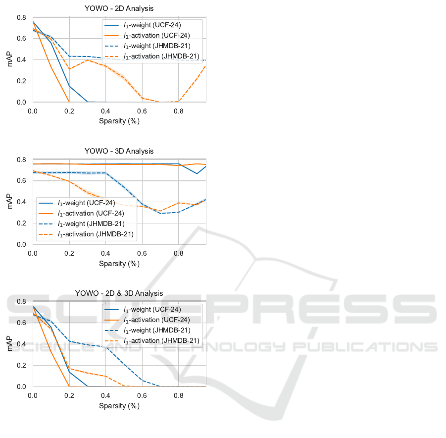
model. In the Figure 4c, we present the results of

the global sensitivity analysis after pruning both the

2D and 3D backbone of the model. It is evident that

the model is signiﬁcantly affected by structured prun-

ing, resulting in a noticeable decrease in performance

to a suboptimal level. Therefore, retraining will be

necessary to achieve higher sparsity levels. Addition-

ally, using the same level of sparsity for both may

be a naive approach. Therefore, we also conducted

a sensitivity analysis for each backbone separately. It

is important to note that in this setting, we leave the

other backbone untouched and still measured the per-

formance of the entire model. The results are shown

in Figure 4a and Figure 4b.

These graphs, conﬁrm our hypothesis that using

the same pruning ratio for both backbones is not opti-

mal. Both backbones react differently to the pruning.

Overall we see that the 2D backbone is more sensi-

tive to pruning than the 3D backbone. This is logical

as the 2D backbone will generally be used for the lo-

calization of the activity instance.

Additionally, we observe that the 3D backbone is

less affected by low sparsity levels. This is partly due

to the architecture used in this backbone (ResNext-

101), which employs channel grouping in its convo-

lutional layers. Channel grouping divides the input

channels into groups and performs separate computa-

tions on each group using separate kernels. For ex-

ample, if a layer has 128 input channels and grouping

is set to 32, the layer will use only four sets of ker-

nels. This means the number of channels to remove is

very limited and will have a signiﬁcant impact on the

model. The model is only impacted when the prun-

ing ratios are high enough, for example at least 25%

in this example. Therefore, for pruning the 3D back-

bone, we use higher pruning ratios than for the 2D

backbone.

Finally, we observe a signiﬁcant difference in sen-

sitivity between datasets. In our experiments, the

model trained on UCF-24 is barely impacted when

we prune the 3D backbone. However, with the model

trained on JHMDB-21, we see a noticeable decrease

in performance. We believe this disparity is due to

the nature of the datasets. As such, a separate pruning

schedule will be needed for each dataset.

In the next section, we will use these results to

make an informed decision on setting up a pruning

schedule for compressing the model.

4.2 Combined Compression Results

In this section we show the results of the com-

bined (pruning and quantization) compression of the

YOWO model. As mentioned previously, we use an

iterative pruning schedule with ﬁne-tuning to prune

the model. We prune the YOWO model in two sep-

arate stages: the ﬁrst stage involves pruning the 2D

backbone, while the second stage involves pruning

the 3D backbone. After each iteration within each

stage, a ﬁne-tuning step is performed. This ﬁne-

tuning is done using the same hyperparameters as the

original training, except for the number of epochs.

From the sensitivity analysis (4.1), we conclude that

pruning the network separately has less impact on the

VISAPP 2024 - 19th International Conference on Computer Vision Theory and Applications

580

(a)

(b)

(c)

Figure 4: The graphs demonstrate the impact of pruning by

assessing the model’s (frame) mAP with increasing sparsity.

(a) displays the sensitivity analysis when pruning the 2D

backbone. (b) displays the sensitivity analysis when prun-

ing the 3D backbone. (c) displays the sensitivity analysis

when pruning both the 2D and 3D backbone.

model’s performance. Using the results of the sensi-

tivity analysis, we set up a pruning schedule for the

full compression pipeline. This schedule is then fur-

ther tuned experimentally. We show the results of the

compression using different pruning schedules. The

schedule is deﬁned by the pruning ratio per step and

for each backbone, the number of steps for each back-

bone and the number of epochs used for ﬁne-tuning.

The different scheduling settings used for the results

presented in this section can be found in section 5 in

the appendix.

The compression results can be found in Table 1.

This table contains the results for the pruning and

quantization of the YOWO model on the JHMDB-21

dataset and the UCF-24 dataset. We show the results

for different pruning schedules with their quantized

counterparts.

These results show a considerable reduction of the

model size and number of operations are achieved.

Overall we are able to generate the smallest models

using the activation based pruning. However, this is

very dataset/task dependent. For the UCF-24 dataset,

we are able to maintain the mAP very well using both

pruning criteria. However, for this dataset the activa-

tion based pruning is able to generate slightly smaller

and faster models. For the JHMDB-21 dataset, we see

a bigger drop in mAP, as this model is more sensitive

to pruning. For this dataset we are not able to com-

press as aggressively. For the results on the JHMDB-

21 we targeted a theoretical speedup of at least two,

while maintaining an acceptable mAP. For the UCF-

24 dataset we targeted a theoretical speedup of at least

four.

Please note that this does not apply to the

JHMDB-21 model with ID 3. For this model we see

an increase of the mAP when pruning the 2D back-

bone using the activation based criterion. In this case,

the model was not pruned too aggressively, which, in

combination with the ﬁne-tuning, resulted in a bet-

ter performing model. This also follows the results

of (Bartoldson et al., 2020) who show that pruning

can be used during training to improve generalization.

Overall, we managed to speed up the model by at

least a factor of two while maintaining an acceptable

mAP score. For the UCF-24 dataset, we (theoreti-

cally) speed up the model by a factor of 6.6, reducing

the mAP by only about 4%. Observing the combined

pruned and quantized results, we found that the gener-

ated models are approximately six times smaller than

the original model. This signiﬁcant size reduction is

highly beneﬁcial for edge deployment. The small-

est models were achieved for the JHMDB-21 dataset.

We can conclude that the most substantial size im-

pact occurs when pruning the 2D backbone more ag-

gressively, as demonstrated by the JHMDB-21 mod-

els. The largest impact on speedup is achieved when

pruning the 3D backbone, as shown by the UCF-24

pruned models.

4.3 Resource Consumption on the

Raspberry Pi 4 Model B

In this section, we present the results of resource

consumption measurements from running the com-

pressed model on the Raspberry Pi 4 Model B. The re-

Deep Learning Model Compression for Resource Efﬁcient Activity Recognition on Edge Devices: A Case Study

581

Table 2: Results of the resource consumption measurements on the Raspberry Pi 4 Model B. We show the results of the

original model trained on the UCF-24 dataset, the activation pruned model (ID: 9) and the quantized version of the activation

pruned model. The latency is the average time it takes to process a single iteration. The runtime memory is the average

memory usage of the model during inference. The energy consumption is the total energy consumption of the model during

inference during the measurement period. The results are gathered by running each model for 100 iterations and measuring

the resource consumption during this period. The average power consumption is measured by running each model at a ﬁxed

framerate of 3.2.

Pruned Quantized Latency (ms) Runtime Memory (MB) Energy Consumption (J) Avg. Power Consumption (W)

✗ ✗ 4381.91 678.13 2032.20 4.19

✓ ✗ 1345.98 450.46 638.27 2.70

✓ ✓ 8583.75 408.16 2774.22 3.04

source consumption is assessed by measuring latency,

memory usage, energy consumption, and power con-

sumption when running inference of the models. We

then compare these results with those of the uncom-

pressed model. Latency and memory usage are mea-

sured using built-in Python tools, while energy con-

sumption is measured with a JouleScope JS110. The

JouleScope measures current and voltage to compute

power and energy. The ﬁndings are summarized in

Table 2.

We measure a model’s latency, memory usage and

energy consumption by running the model for a ﬁxed

number of iterations. It’s important to note that the

duration of this experiment can vary, as compressed

models operate faster than their uncompressed coun-

terparts. The CPU operates at full capacity continu-

ously, which means there is no difference in power

consumption between models when working in this

mode. It is due to the lower number of operations that

the compressed models are faster and consume less

energy. In a real-world scenario, the models would

run in a ﬁxed number of iterations per second (or

framerate) mode. In this case, compressed models

would idle the CPU for extended periods, resulting

in power and energy savings. We evaluated the to-

tal energy consumption, average latency, and average

memory usage of the model over 100 iterations with-

out a limitation on the framerate. The average power

consumption was measured in a separate experiment

by running each model at a ﬁxed framerate of 3.2 for

the same number of iterations.

We observe that pruning has the most signiﬁcant

impact on the models. It signiﬁcantly reduces the en-

ergy consumption by 69% and power consumption by

36%, while making the model 3.3 times faster. How-

ever, there’s a notable difference between the theoret-

ical speedup (5.62) and the actual measured speedup.

We attribute this discrepancy to factors like the sched-

uler, memory access delays, and general background

tasks of the operating system.

Additionally, while quantization does improve

memory, it unfortunately worsens latency and energy

consumption. This is primarily due to the software

limitations of the Raspberry Pi. Currently, the used

ONNX runtime and its execution providers do not

support 3D convolutions in quantized mode. This

could be improved in future work.

5 CONCLUSION AND FUTURE

WORK

In this work, we investigate the feasibility of deep

learning-based activity recognition on edge devices.

More speciﬁcally, we investigate the compression the

YOWO model proposed by (K

ukl

u et al., 2019).

This model has a single-stage architecture consist-

ing of two branches: a 2D backbone and a 3D back-

bone. This architecture is very large, consisting of

millions of parameters and requiring billions of op-

erations, making it too large and complex for edge

deployment.

We propose a two-stage compression approach:

structured channel pruning and quantization. By ap-

plying iterative structured channel pruning, we aim to

reduce the size and the number of operations of the

YOWO model while maintaining its accuracy. This

pruning technique removes the least important chan-

nels from the network. We compare two importance

criteria, namely, the weight magnitude and the acti-

vation magnitude. Additionally, we combine prun-

ing with quantization, further reducing the size of

the model by representing the weights and activations

with fewer bits.

To evaluate the effectiveness of our approach, we

deploy the compressed YOWO model on the Rasp-

berry Pi 4 Model B and measure its latency, mem-

ory usage, energy and power consumption. The

compressed models were generated after a sensitiv-

ity analysis to determine the impact of pruning the

YOWO models and to ﬁnd the optimal parameters

for scheduling the pruning. The results of the com-

bined pruning and quantization approach show that

we can signiﬁcantly reduce the size and operations

of the YOWO model while maintaining task perfor-

VISAPP 2024 - 19th International Conference on Computer Vision Theory and Applications

582

mance. For the UCF-24 dataset, we are able to speed

up (theoretically) the model by a factor of 6.6 while

only reducing the mAP by about 4%.

This result can also be observed in the energy con-

sumption, where there’s a reduction by a factor of

3.2. This signiﬁcant decrease is especially vital con-

sidering energy consumption is a crucial factor for

edge deployment, enabling the model to be utilized on

battery-powered devices. By examining the memory

usage and latency of the deployed models, it’s clear

that the compressed models are more suitable for edge

deployment.

For future work, other pruning criteria and

scheduling methods can be investigated. Currently,

we used sensitivity analysis to determine a pruning

schedule. However, this is not the optimal way to de-

termine the schedule. This could potentially be au-

tomated, as done in the ﬁeld of AutoML. For exam-

ple, in the work of (He et al., 2018), a reinforcement

learning approach is used. Furthermore, we used a

static post-training quantization method. In future

work, we could investigate the use of quantization-

aware training. Finally, the quantization results can

also be improved by better software support, as dis-

cussed in Section 3.3.

ACKNOWLEDGEMENT

This research is partly supported by the FWO

SBO Fellowship 1SA8124N ”Knowledge Based Neu-

ral Network Compression: Context-Aware Model

Abstractions” and by the Flanders Innovation En-

trepreneurship (VLAIO) IMEC.ICON project no.

HBC.2021.0658 BoB.

REFERENCES

Bartoldson, B., Morcos, A., Barbu, A., and Erlebacher, G.

(2020). The generalization-stability tradeoff in neu-

ral network pruning. In Larochelle, H., Ranzato,

M., Hadsell, R., Balcan, M. F., and Lin, H., editors,

Advances in Neural Information Processing Systems,

volume 33, pages 20852–20864. Curran Associates,

Inc.

Braun, A., Tuttas, S., Borrmann, A., and Stilla, U.

(2020). Improving progress monitoring by fusing

point clouds, semantic data and computer vision. Au-

tom. Constr., 116:103210.

Crowley, E. J., Turner, J., Storkey, A., and O’Boyle, M.

(2018). A closer look at structured pruning for neural

network compression. pages 1–12.

Feichtenhofer, C., Fan, H., Malik, J., and He, K. (2018).

SlowFast networks for video recognition.

Feichtenhofer, C., Pinz, A., and Zisserman, A. (2016). Con-

volutional Two-Stream network fusion for video ac-

tion recognition.

Frankle, J. and Carbin, M. (2018). The lottery ticket hypoth-

esis: Finding sparse, trainable neural networks. pages

1–42.

Georgiadis, G. (2018). Accelerating Convolutional Neu-

ral Networks via Activation Map Compression. Pro-

ceedings of the IEEE Computer Society Conference

on Computer Vision and Pattern Recognition, 2019-

June:7078–7088.

Han, S., Mao, H., and Dally, W. J. (2016). Deep compres-

sion: Compressing deep neural network with pruning,

trained quantization and huffman coding. In 4th In-

ternational Conference on Learning Representations,

ICLR 2016, San Juan, Puerto Rico, May 2-4, 2016,

Conference Track Proceedings.

He, Y., Lin, J., Liu, Z., Wang, H., Li, L.-J., and Han, S.

(2018). AMC: AutoML for model compression and

acceleration on mobile devices.

He, Y., Zhang, X., and Sun, J. (2017). Channel pruning for

accelerating very deep neural networks. In 2017 IEEE

International Conference on Computer Vision (ICCV),

volume 2017-Octob, pages 1398–1406. IEEE.

IMEC (2023). imec.icon project - BoB. https://www.

imec-int.com/en/research-portfolio/bob. Accessed:

2023-11-13.

Jacob, B., Kligys, S., Chen, B., Zhu, M., Tang, M., Howard,

A., Adam, H., and Kalenichenko, D. (2017). Quan-

tization and training of neural networks for efﬁcient

Integer-Arithmetic-Only inference.

Jhuang, H., Gall, J., Zufﬁ, S., Schmid, C., and Black, M. J.

(2013). Towards understanding action recognition. In

2013 IEEE International Conference on Computer Vi-

sion, pages 3192–3199. IEEE.

ukl

u, O., Wei, X., and Rigoll, G. (2019). You only

watch once: A uniﬁed CNN architecture for Real-

Time spatiotemporal action localization.

Krishnamoorthi, R. (2018). Quantizing deep convolutional

networks for efﬁcient inference: A whitepaper.

Kuehne, H., Jhuang, H., Garrote, E., Poggio, T., and Serre,

T. (2011). HMDB: A large video database for human

motion recognition. In 2011 International Conference

on Computer Vision, pages 2556–2563. IEEE.

Lee, N., Ajanthan, T., and Torr, P. H. S. (2018). SNIP:

single-shot network pruning based on connection sen-

sitivity. CoRR, abs/1810.02340.

Li, H., Kadav, A., Durdanovic, I., Samet, H., and Graf,

H. P. (2016). Pruning Filters for Efﬁcient ConvNets.

5th International Conference on Learning Represen-

tations, ICLR 2017 - Conference Track Proceedings,

(2016):1–13.

Liu, C. and Wu, H. (2019). Channel pruning based on

mean gradient for accelerating Convolutional Neural

Networks. Signal Processing, 156:84–91.

Loshchilov, I. and Hutter, F. (2017). Decoupled weight de-

cay regularization.

ONNX (2023). Open neural network exchange. https://

onnx.ai/. Accessed: 2023-11-13.

Deep Learning Model Compression for Resource Efﬁcient Activity Recognition on Edge Devices: A Case Study

583

Qiu, Z., Yao, T., and Mei, T. (2017). Learning Spatio-

Temporal representation with Pseudo-3D residual net-

works.

Redmon, J. and Farhadi, A. (2016). YOLO9000: Better,

faster, stronger.

Simonyan, K. and Zisserman, A. (2014). Two-Stream con-

volutional networks for action recognition in videos.

Soomro, K., Zamir, A. R., and Shah, M. (2012). UCF101:

A dataset of 101 human actions classes from videos in

the wild.

Tanaka, H., Kunin, D., Yamins, D. L. K., and Ganguli, S.

(2020). Pruning neural networks without any data by

iteratively conserving synaptic ﬂow.

Tran, D., Bourdev, L., Fergus, R., Torresani, L., and Paluri,

M. (2014). Learning spatiotemporal features with 3D

convolutional networks.

Tran, D., Wang, H., Torresani, L., Ray, J., LeCun, Y., and

Paluri, M. (2017). A closer look at spatiotemporal

convolutions for action recognition.

Wen, W., Wu, C., Wang, Y., Chen, Y., and Li, H. (2016).

Learning structured sparsity in deep neural networks.

Xie, S., Girshick, R., Doll

ar, P., Tu, Z., and He, K. (2016).

Aggregated residual transformations for deep neural

networks.

A Appendix

A.1 Scheduling Hyperparameters

In Table 3 the different scheduling hyperparameters used for

the pruning experiments are shown. These settings where

chosen based on the results of the sensitivity analysis and

experimentally tuned.

A.2 Training Hyperparameters

In this section the different training hyperparameters used

for the experiments are shown. We utilized two different

datasets to train the base models for compression. Table 4

lists the hyperparameters used for training these base mod-

els.

Table 4: Training Hyperparameters for UCF-24 and

JHMDB-21 datasets.

Dataset UCF-24 JHMDB-21

Parameter

Downsample 1 1

Temporal Downsample 2 1

Clip Length 16 16

Conﬁdence Threshold 0.3 0.3

NMS Threshold 0.5 0.5

Conﬁdence Threshold (Validation) 0.005 0.005

NMS Threshold (Validation) 0.5 0.5

Freeze 2D Backbone False False

Freeze 3D Backbone False False

Batch Size 8 4

Test Batch Size 8 8

Accumulate 16 16

Optimizer adamw adamw

Momentum 0.9 0.9

Weight Decay 0.0005 0.0005

Max Epoch 5 5

Base Learning Rate 0.0001 0.0001

Learning Rate Decay Ratio 0.5 0.5

Warmup Strategy linear linear

Warmup Factor 0.000667 0.000667

Warmup Iterations 500 500

Table 3: Different scheduling hyperparamters used for the pruning for the in the full compression pipeline.

ID Dataset Attribution 2D Iterations 3D Iterations 2D Pruning Ratio 3D Pruning Ratio Fine-tuning Epochs

0 JHMDB-21 — — — — — —

1 JHMDB-21 weight 1 4 0.90 0.60 6

2 JHMDB-21 weight 5 8 0.50 0.80 5

3 JHMDB-21 activation 5 0 0.50 — 5

4 JHMDB-21 activation 1 4 0.90 0.60 6

5 JHMDB-21 activation 5 2 0.50 0.80 5

6 UCF-24 — — — — — —

7 UCF-24 weight 0 12 0.00 0.90 6

8 UCF-24 weight 1 12 0.20 0.90 6

9 UCF-24 activation 0 12 0.00 0.90 6

10 UCF-24 activation 1 12 0.20 0.90 6

VISAPP 2024 - 19th International Conference on Computer Vision Theory and Applications

584