Hierarchical Bitmask Implicit Grids for Efﬁcient Point-in-Volume

Queries on the GPU

Julius Ikkala

, Tuomas Lauttia

, Pekka J

askel

ainen

and Markku M

akitalo

Tampere University, Tampere, Finland

ﬁ

Keywords:

Computer Graphics, Real-Time Rendering, Ray Tracing, Data Structures.

Abstract:

We propose “Hierarchical Bitmask Implicit Grids”, a novel, memory-efﬁcient spatial index data structure

for querying bounding volumes based on a contained point, targeting real-time use cases on GPUs. Like

grid structures based on 3D arrays, implicit grids allow for nearly array-like direct lookups of cells without

traversal through a spatial tree structure. However, the space complexity of this structure is O(n) with respect

to resolution as opposed to O(n

), which allows for dramatically higher resolutions than would be feasible

with a 3D array. We demonstrate the effectiveness of this data structure by applying it to two example use

cases: light culling and decal rendering. We measure both cases with ray tracing and multi-view rendering.

We show that with tens of thousands of entries, our data structure can be built in 0.1–0.2 milliseconds, being

∼2.9x faster than the compared state-of-the-art decal method and orders of magnitude faster than dense 3D

arrays, while delivering at least similar or even up to doubled rendering performance.

1 INTRODUCTION

Looking up overlapping volumes for a point in space

is a common problem in real-time computer graphics.

Two typical examples of this encountered in modern

video games are light culling, i.e. ﬁguring out which

limited set of lights are taken into account when shad-

ing a surface; and decals, which modify the mate-

rial data at a surface in order to add things like bul-

let holes and puddles, often dynamically. (Akenine-

oller et al., 2018)

These problems are typically solved with highly

efﬁcient screen-space structures (Olsson and Assars-

son, 2011; Geffroy et al., 2020). However, the screen-

space domain does not include points outside of the

view frustum, which are commonly encountered with

ray tracing, as rays can freely bounce within the

scene. For multi-view displays, screen-space struc-

tures would be calculated for each view separately,

multiplying their build time by however many views

are needed. For example, the Looking Glass Portrait

display usually takes between 48–100 separate views

in its ”quilt” (Looking Glass Factory, Inc., 2023).

Even a 0.1 ms build time for a single view can there-

https://orcid.org/0000-0002-5373-3190

https://orcid.org/0000-0003-3568-6316

https://orcid.org/0000-0001-5707-8544

https://orcid.org/0000-0001-8164-0031

fore balloon to 5 to 10 milliseconds, which is a signif-

icant portion of the 16 milliseconds available in a 60

Hz target framerate.

Both issues with ray tracing and multi-view dis-

plays can be alleviated by using a world-space data

structure. Several contemporary game engines are us-

ing grids based on 3D arrays (Unity Technologies,

2023; Kelly et al., 2021) to cull light sources for ray

tracing. These have fast lookup times: the lookup

is simply accessing an array, unlike tree structures,

which traverse through a hierarchy of nodes with data

dependencies between each step. The downside to 3D

arrays is the space complexity of O(n

), which makes

high-resolution or large-scale grids impractical. Vary-

ing grid cell sizes based on camera distance alleviates

this problem somewhat in practice (Kelly et al., 2021),

at the expense of precision at distance.

As an improvement over 3D arrays, we propose a

world-space data structure for querying a list of vol-

umes overlapping with a given point in space. It is

an implicit grid; the cells are only constructed during

lookup by combining per-axis information. The im-

plicit grid is sliced into slabs along each of the three

principal axes. The overlap status of each entry’s vol-

ume is stored in a bitmask with each slab. Given a

point, taking the bitwise AND of the bitmasks of cor-

responding slabs yields a set of overlapping volumes

with no false negatives.

Ikkala, J., Lauttia, T., Jääskeläinen, P. and Mäkitalo, M.

Hierarchical Bitmask Implicit Grids for Efﬁcient Point-in-Volume Queries on the GPU.

DOI: 10.5220/0012421600003660

Paper published under CC license (CC BY-NC-ND 4.0)

In Proceedings of the 19th International Joint Conference on Computer Vision, Imaging and Computer Graphics Theory and Applications (VISIGRAPP 2024) - Volume 1: GRAPP, HUCAPP

and IVAPP, pages 285-292

ISBN: 978-989-758-679-8; ISSN: 2184-4321

285

The bitmasks are very sparse when there are thou-

sands of small volumes in a large scene. To take

advantage of this sparsity, we propose a hierarchical

layer which allows skipping over large empty portions

in the bitmasks, improving lookup time signiﬁcantly.

With the bitmask sizes we suggest, just one layer of

hierarchy is effective for up to at least tens of thou-

sands of entries. We further increase the effectiveness

of this hierarchical structure by sorting the entry vol-

umes along the Z-order curve (Morton, 1966) before

building the acceleration structure.

In practice, we demonstrate that on contemporary

GPU hardware, this data structure is efﬁcient to build

from scratch, even with up to tens of thousands of

entries. Further, we show that our data structure is

highly effective for its typical use cases: light culling

and decal lookup in multi-view rasterization and ray

tracing. In this article, we present the following con-

tributions:

• Application of implicit grids to light culling in ray

tracing and multi-view contexts.

• Application of implicit grids to decal rendering in

ray tracing and multi-view contexts.

• Addition of a hierarchical layer and Z-order curve

sorting to implicit grids for improving the lookup

performance.

2 RELATED WORK

Tiled Deferred Shading and Tiled Forward Shading

(Balestra and Engstad, 2008; Olsson and Assarsson,

2011) cull lights with a contribution below a given

threshold by dividing the screen into tiles and assign-

ing the kept lights to each tile. Clustered deferred and

forward shading (Olsson et al., 2012) improve on this

by presenting a method that also divides the tile frusta

into cells (called clusters) by depth. Compared to

tiled shading, this method lets fewer lights be handled

within screen-space tiles with great depth discontinu-

ities. Similar data structures have also been used for

decal rendering in forward pipelines (Geffroy et al.,

2020). However, these screen-space structures are

not generally applicable to ray tracing, as they only

cull data within the viewport, while bounced rays can

reach out-of-screen areas as well. Multi-view render-

ing would also require building these for each view-

point, making the build time of screen-space struc-

tures less than ideal in that case.

World-space light clustering methods have been

limited to naive dense grids in the industry (Unity

Technologies, 2023; Kelly et al., 2021). The cubic

space complexity of these grids forces them to be

quite low-resolution. (Kelly et al., 2021) uses varying

cell sizes in the grid structure, based on camera posi-

tion. We use uniform cell sizes, as the implicit data

structure allows for enough precision with a compact

memory footprint to simply increase resolution glob-

ally whenever precision is not high enough near the

camera.

(Bahnassi, 2021) present methods for ﬁnding de-

cals in world-space by placing their bounding vol-

umes in a Top-Level Acceleration Structure (TLAS)

and tracing effectively zero-length rays. Their most

performant variant that supports multiple overlapping

decals is based on using an any-hit shader to collect

a list of decals. They suggest using a small array for

this, e.g. 2-3 entries. Having more overlapping decals

than that will cause issues with this method, appear-

ing as unpredictable decal ordering and missing de-

cals. They also present a variant which does not have

this limitation, but it is an order of magnitude slower

according to their measurements.

Our proposed method has similarities to collision

detection methods: the sweep-and-prune algorithm

(also known as sort-and-sweep) (Baraff, 1992) uses a

similar approach in which objects are bound by over-

lapping slabs along axes. However, that method di-

vides the axes continuously and cannot do individ-

ual coverage lookups in constant time. The basic

bitmask-based implicit grid data structure itself is not

new: (Ericson, 2005) introduced a form of it for use

in collision detection (implicit grid using bit arrays).

Another data structure with similarities has been

proposed in the context of light culling for rasteriza-

tion by (Drobot, 2017). Their light clustering method

separates the Z axis from the X and Y axis with “Z-

binning” and also uses bitmasks. Based on this, a

blog post (Sylvan, 2017) suggested binning X and Y

axes as well. This would have resulted in a similar

data structure as the one described by (Ericson, 2005).

However, the author admits in the post that they did

not implement or evaluate the method.

To our knowledge, the implementation of this data

structure in this ﬁeld and the hierarchical layer are

novel contributions. Compared to grids based on 3D

arrays, implicit grids improve on the space complex-

ity, from O(n

) to O(n) where n is the number of grid

cells along an edge. The hierarchical layer improves

iteration speed in situations with tens of thousands of

entries by allowing skipping large portions of the bit-

mask at once.

GRAPP 2024 - 19th International Conference on Computer Graphics Theory and Applications

286

0 0 0 0

1 1

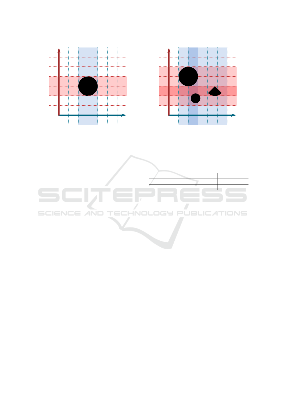
(a) One object. A set bit signals presence on a slab.

001

011

110

010

010 100 100000

000

(b) For multiple objects, there is one bit per object.

Figure 1: A 2D analog of the data structure. The bitmasks on each slab specify which objects overlap with the slab. The least

signiﬁcant bit corresponds to object 1. The bitwise-AND of the bitmasks of two slabs corresponding to any grid cell results

in a bitmask representing the set of objects which potentially overlap with the cell.

3 IMPLICIT GRID

The proposed implicit grid data structure works by

storing the effective range of each object along three

axes. The axes are sliced into evenly spaced slabs.

Each slab is represented by a bitmask. A slab bit-

mask has one bit per object, which is set to 1 if the

object overlaps with this slab and 0 if not. To de-

termine which objects overlap with a given grid cell

in space, a bitwise AND of the bitmask of the cor-

responding slab on each axis is taken. The objects

which potentially overlap with the grid cell are set to

1 in the resulting bitmask. Due to the nature of us-

ing three perpendicular axes in this data structure, the

shape of the volume bounding an object is an axis-

aligned rectangular cuboid, so the structure will report

false positives if the true shape of the range is some-

thing else. Figure 1a visualizes the implicit grid with

a single object, while Figure 1b shows a multi-object

situation.

Compared to explicit grids, this method is both

cache friendly and memory efﬁcient (Ericson, 2005);

the data needed to look up a grid cell is always near its

world-space neighbors in memory as well, due to each

axis being stored as a linear list of bitmasks. Addi-

tionally, the memory usage and build time is O(3mn)

instead of O(mn

), where m is the number of entries

and n is the number slabs on every axis. Both beneﬁts

map well to modern GPU architectures as well.

In practice, we store the per-slab bitmask as an

array of 4-channel vectors of 32-bit unsigned inte-

gers. We selected this vector width by also testing

2-channel 32-bit vectors and 4-channel 64-bit vectors,

and found the 4-channel 32-bit approach fastest in our

Table 1: An example of a hierarchical bitmask layer, with

sector size of 4 bits. The hierarchical layer can be used to

quickly skip large portions of the full bitmask.

Entry indices 16-13 12-9 8-5 4-1

Full bitmask 0000 0000 1100 0101

Hierarchy layer 0 0 1 1

implementation, on an RTX 3090. Other sizes could

very well be optimal on some other hardware or use

cases. Since these parameters do not affect the output

image in any way, the optimal parameters can be cho-

sen by selecting whichever is fastest on the hardware

in question. A 4-channel vector of 32-bit integers has

128 bits, and can thus represent the presence of 128

entries. We call these vectors “bitmask sectors” going

forward.

3.1 Hierarchy

Once the number of entries is high enough (typically

in the tens of thousands), directly iterating through

all bitmask sectors becomes costly. Most of the bit-

mask sectors are usually empty, as entries generally

only cover a small portion of the entire scene. To re-

duce the number of reads needed to iterate through

the set bits of the bitmask, we use another bitmask as

a layer of hierarchy. The bits of this hierarchical bit-

mask layer represent each sector of the base bitmask.

A bit is set to 1 if any of the bits in the corresponding

sector is 1. This way, bitmask sectors fully consist-

ing of zero can be quickly skipped. Table 1 shows an

example case of this.

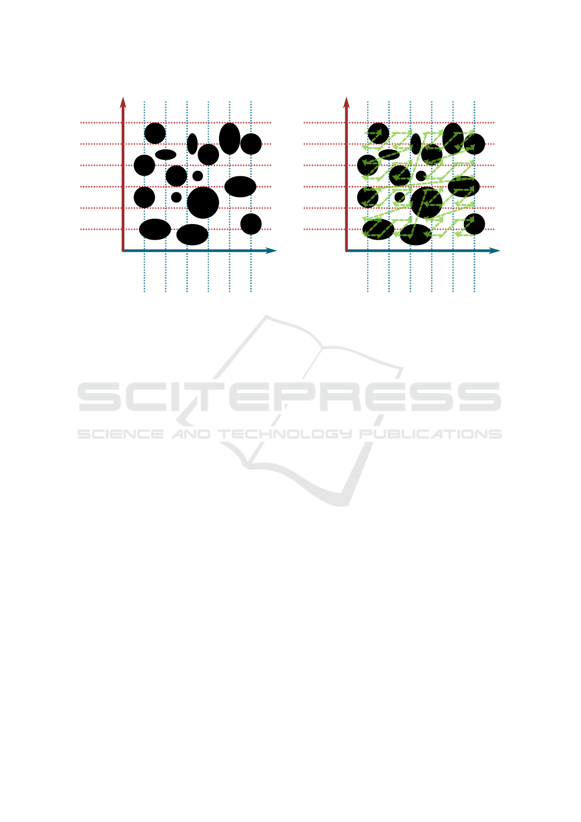
Even if the bitmasks are mostly sparse, if the order

of entries is random, the bits are spread throughout

Hierarchical Bitmask Implicit Grids for Efﬁcient Point-in-Volume Queries on the GPU

287

the sectors uniformly, causing many bitmask sectors

to have just a few bits set. The hierarchy is most ef-

fective when as many sectors as possible are fully zero

and thus skippable, with the 1-bits mostly present to-

gether in individual sectors. Sorting the entries ac-

cording to the Z-order curve (Morton, 1966) before

building the implicit grid drastically improves the ef-

ﬁciency of the hierarchy, due to grouping nearby en-

tries in the same or nearby bitmask sectors. Figure 2

visualizes the effect of this sorting.

We calculate the Z-order curve inside the axis-

aligned bounding box (AABB) that contains the cen-

troids of all objects, and sort based on the centroid lo-

cation. We use 10-bit precision per axis in the curve,

as it was the maximum precision we could ﬁt in a

32-bit index (3 axes times 10 bits). Lower precision

can also be used, but doing so can reduce the beneﬁt

gained by sorting when the resolution of the Z-order

curve is lower than the density of slabs in the grid.

3.2 Building

The process of building the implicit grid consists of

the following steps:

1. (Optional) Sort volumes by centroid coordinate

along Z-order curve

2. Calculate applicable range of each volume along

each axis

3. For each bitmask sector of each slab of each axis,

ﬁnd overlapping volume ranges and assign bits

4. (Optional) Build hierarchical bitmask layer based

on high-resolution bitmasks.

The building process can be fully implemented on

the GPU, and the steps past sorting are “embarrass-

ingly parallel”.

We implement step 1 using a Vulkan-based radix

sort implementation (The Fuchsia Authors, 2021). In

practice, we used a 30-bit Z-order curve, 10 bits per

axis. The curve is aligned to the AABB containing

the centroids of all volumes. The sorting is used to

roughly cluster lights with similar overlaps into suc-

cessive bits; this makes the hierarchical bitmask layer

more effective at skipping sectors due to more sectors

being completely zero. If the hierarchical layer is not

used, this speciﬁc beneﬁt no longer applies and sort-

ing can thus be skipped without major performance

implications.

When handling step 2 in the light culling context,

the range of each light is initially estimated based on a

cut-off brightness parameter. During step 2, the struc-

ture can take visibility into account for a fairly low

additional cost. If shadow maps have been computed

for each light source, the ranges can be bounded by

the maximum AABB of the distances present in each

shadow map. Decals, on the other hand, are typically

already deﬁned as Oriented Bounding Boxes (OBB);

the range step only needs to ﬁnd the extents of the

OBB along each grid axis (i.e. ﬁnd the AABB con-

taining the decal OBB).

For step 3, we use a workgroup geometry of

32×4, representing 32 slabs and the 4 32-bit unsigned

integers forming a sector. Each work item reads one

range into shared memory, corresponding to the 128

bits in the current sectors. This way, the range infor-

mation needed to build the bitmasks for 32 slabs can

be fetched at once. The rest of the step is trivial: on

each slab, go through the light ranges for the sector,

and write a 0 or 1 bit to the bitmask depending on if

the range overlaps with the bitmask’s slab.

Step 4, the hierarchical layer, is optional, and usu-

ally only beneﬁcial when the number of entries is in

the thousands. It is built in a quite simple manner: for

each bit in the hierarchical layer, read the sector from

the full bitmask, and check if it is non-zero.

3.3 Iterating over Entries

First, the queried point’s coordinate is transformed

and quantized to the location and resolution of the im-

plicit grid. The resulting coordinates on each axis cor-

respond directly to the slab indices. When not utiliz-

ing the hierarchical layer, we then iterate through the

bitmasks of the selected slabs, calculate the bitwise

AND between them, and report the index of each set

bit as an overlap.

As a concrete example, in the decal rendering

case, if the queried point is the position of the surface

depicted in a given pixel, then the reported indices

correspond to decals which are potentially present at

the surface.

In the case with a hierarchy, we ﬁrst iterate

through the hierarchy bitmask in a similar bitwise

AND fashion. Instead of reporting the index when a

set bit is encountered, we instead now visit the corre-

sponding sector in the underlying bitmask and calcu-

late the bitwise AND between those slabs and report

those indices.

4 EXPERIMENTAL SETUP

We apply the proposed hierarchical bitmask implicit

grid (HBIG) data structure to two different use cases:

decal rendering and light culling. In both situations,

we use a PBR version of the “Sponza” scene (The

Khronos Group, 2018) with added relevant elements,

as shown in Figure 3. We set our implicit grid imple-

GRAPP 2024 - 19th International Conference on Computer Graphics Theory and Applications

288

1 6

0000 1000

0010 0011

0100

0011

0100

0010

0100

0010

0100

0000

0011

0001

0101

0000

1010

0000

1000

1001

1000

0100

0000

1100

0010

0100

0000

0100

0010

0100

1000 1011

0010 0001

0001 0010

0000 1100

0100

0000

1001 0100

0010 0100

1100 0000

0010 0100

0100 0000

(a) The objects are in random order.

0000 0000

1100 0101

0000 0000

1110 1110

0100 0001

0001 1000

0110 0110

0000 0000

1011 1000

0000 0000

1001 1000

0000 0000

0000

1010

0000

1000

0000

1010

0000

1011

0001

1100

0001

0010

0011

0001

0010

0100

0110

0000

0110

0000

1100

0000

1100

0000

1100

0000

1000

0000

(b) The new indices assigned along a Z-order curve.

Figure 2: A 2D analog of the data structure, showing bitmasks in a 16-object situation. In each bitmask, the top-left bit

corresponds to object 16, while the bottom-right corresponds to 1. (a) The objects are in random order. As the indices

for each bitmask are mostly uniformly distributed, it is rare for 4-bit sectors to be fully zero. (b) The indices have been

assigned along the Z-order curve. As ordering the objects according to their location also places them near each other in the

bitmask, they are more likely to appear in the same sector. This increases the number of empty sectors, which in turn lets the

hierarchical bitmask layer skip more entries.

mentation to start using the hierarchy layer and entry

sorting at 1024 entries, as they have little to no beneﬁt

before that. In all cases, we use a resolution of 512

for all implicit grids.

For decal rendering, we measure performance by

spreading a range of 0 to 65536 decals across the sur-

faces of the test scene at random, as seen in Figure 3a.

In this case, the scene is lit by one bright light source.

We compare our method to a decal rendering method

based on using the Top-Level Acceleration Structure

(TLAS) for querying the bounding boxes of decal vol-

umes (Bahnassi, 2021).

The TLAS approach requires special care with

overlapping decals; to be performant, the maximum

number of allowed overlapping decals needs to be

fairly small. However, our test case has several re-

gions with lots of overlaps. We set the maximum

overlap count to 4 to not slow down the algorithm too

much but also allow it to deal with many of the over-

lapping decals, although several areas in the scene

still have some issues due to having 5 or more over-

laps.

For light culling, we spread 0 to 65536 point lights

randomly in the same scene, as seen in Figure 3b. The

lights are kept relatively dim so that for any point in

space, most lights can be culled. This is necessary to

demonstrate the efﬁciency of light culling algorithms.

We compare our method to 3D arrays with links to

light lists. Constant-size cells were used due to the

relatively constrained size of the scene. We present

two cases: 16

(A16) which is faster to build but

causes long light lists due to low granularity, and 32

(A32) which is slower to build but has more precision

to cull lights more accurately.

For both use cases, we measure two contexts:

multi-view rasterization and path tracing. For multi-

view rasterization, we render a 16 × 8 grid of views

at the resolution of 256 × 256, offset from each other

by 0.1 units. This setup is chosen to approximate the

needs of light ﬁeld displays (Looking Glass Factory,

Inc., 2023) while keeping rendering performance in

the real-time territory. For ray tracing with decals, we

path trace one indirect bounce at 1920×1080. For the

light case, we instead calculate shadow rays to each

shaded light, but only if the light is within its range.

This approach limits the performance hit of false pos-

itives. We did not implement similar skipping in the

multi-view case, which thus also visualizes the false

positive rate differences more clearly.

In all cases, we measure the time taken to build

the corresponding data structure, as well as render-

ing time. Build times include sorting when it is be-

ing used, and rendering times include data structure

lookups along with rendering tasks like ray tracing

and rasterization. For each data point, we measure

the times for 100 frames and average them. The mea-

surements are run at increments of 128 entries. They

were run on a PC with an RTX 3090 GPU.

Hierarchical Bitmask Implicit Grids for Efﬁcient Point-in-Volume Queries on the GPU

289

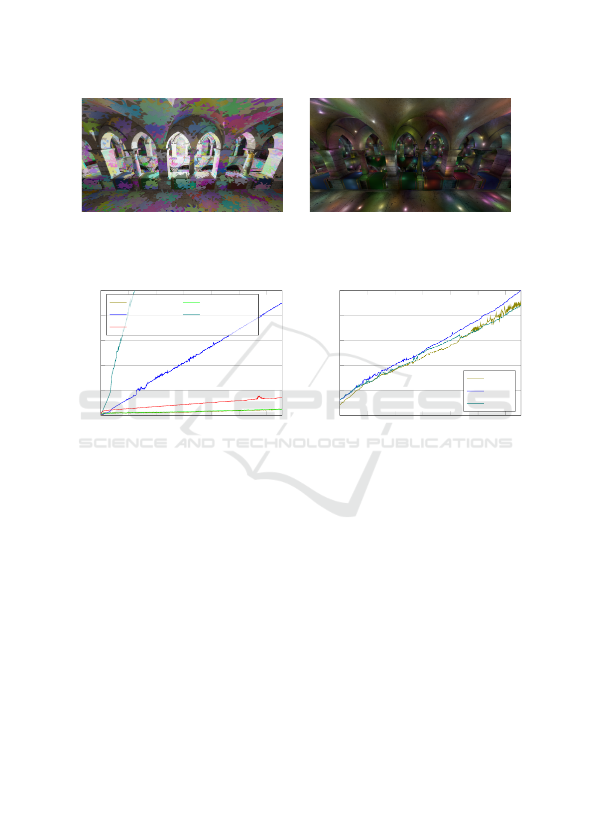
(a) Decal rendering with 65536 decals. (b) Light culling with 65536 lights.

Figure 3: We use the “Sponza” scene in our measurements of both example use cases of implicit grids. We vary the number

of entries from 0 to 65536. When the compared algorithms are functioning correctly, there are no differences in image quality

or contents.

0 1 2 3 4

5 6

·10

Item count

Time (ms)

Build performance

HBIG lights HBIG decals

A16 lights A32 lights

TLAS decals

Figure 4: Performance scaling of the build step of each

method as the number of entries changes.

5 RESULTS

Figure 4 shows the build time of each compared data

structure. The build times between ray tracing and

multi-view runs are essentially identical due to the

workload being the exact same, so we only present

the build times measured from the ray tracing runs.

At 65536 entries, implicit grids only took 0.24 ms to

build in both use cases. The 32

3D array took around

27 ms to build, while 16

took ∼4.5 ms. Building the

decal TLAS took ∼0.7 ms, which is around triple that

of the implicit grid method.

As shown in Figure 5, there are no big differences

in the rendering times between the methods when ray

tracing shadow rays, other than the 16

3D array be-

ing slightly slower at high light counts. This slow-

down is caused by light lists in each cell being larger

than necessary due to the limited precision, resulting

in poor culling. The differences between all of the

methods are small due to shadow rays being skipped

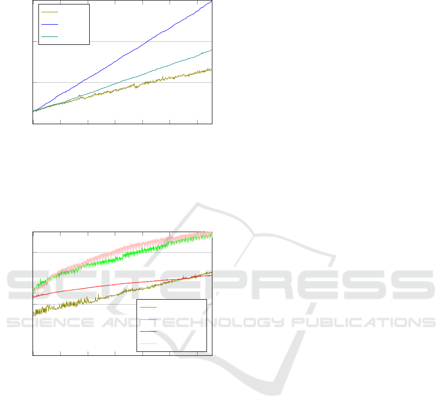
0 1 2 3 4

5 6

·10

Light count

Time (ms)

Rendering, RT light culling

HBIG

A16

A32

Figure 5: Performance scaling of rendering with each

method in the light culling use case in ray tracing. Dif-

ferences are diminished due to shadow rays being skipped

for false-positive lights.

for all “false-positives”; lights that are in range ac-

cording to the data structure but can still be culled

based on their range limit.

In the multi-view rasterization case, we only cull

lights based on the structures themselves, and do

not skip “false-positives” the same way as previ-

ously. Therefore, Figure 6 demonstrates the differ-

ences achieved by better culling precision much more

clearly; with high light counts, implicit grids are over

twice as fast as 16

3D grids and over 25% faster than

Figure 7 shows all decal rendering performance

curves. In the ray tracing use case, implicit grids have

a lower overhead at the low decal counts, but lose

out in the high end as the TLAS case has a shallower

slope. However, the TLAS method renders incorrect

images near the end of the range due to many regions

having more than 4 overlapping decals. This means

that because the implicit grid method is actually cor-

GRAPP 2024 - 19th International Conference on Computer Graphics Theory and Applications

290

0 1 2 3 4

5 6

·10

Light count

Time (ms)

Rendering, MV light culling

HBIG

A16

A32

Figure 6: Performance scaling of rendering with each

method in the light culling use case in multi-view rasteri-

zation. False positives are not skipped in this case, which

shows the beneﬁt of the higher precision achieved with the

implicit grid.

0 1 2 3 4

5 6

·10

Decal count

Time (ms)

Rendering, decals

HBIG RT

HBIG MV

TLAS RT

TLAS MV

Figure 7: Performance scaling of rendering with each

method in the decal rendering use case. The TLAS ap-

proach has disproportionately good results at high decal

counts due to only handling up to 4 overlapping decals cor-

rectly, the rest being skipped if more decals are encountered.

rectly handling all overlapping decals, it is blending

more decals together per pixel than TLAS, causing

more computation and memory accesses.

The multi-view decal case shows both methods

competing closely with each other in the low decal

counts, with implicit grids taking a lead near 2

de-

cals. At that point, stacks of over 4 overlapping de-

cals are rare. As the decal count increases, the TLAS

method catches up to implicit grids but also starts ren-

dering incorrect images for the same reason as in the

ray tracing case.

Table 2 shows building and rendering perfor-

mance differences when the hierarchy layer and sort-

ing of entries are toggled on and off. The order of

entries in the unsorted cases is random. There are

only minor differences between each variation in the

build times; this is expected as the workload of each

build step is the same if the step is present. Rendering

performance is signiﬁcantly hindered if the hierarchy

layer or entry sorting are disabled.

Overall, implicit grids are much faster to build

than any of the other methods at practically every en-

try count. The rendering performance is also either

similar or better than the compared methods in each

situation. In total, the overall cost (build + render) of

implicit grids is lower even in the TLAS comparison

with ray tracing: even if we disregard TLAS’s over-

lap issue, the build time difference of 0.47 ms to the

implicit grid’s beneﬁt is enough to beat TLAS’s ren-

dering time lead of 0.36 ms at 65536 decals.

6 FUTURE WORK

Using the X, Y and Z axes for the implicit grid results

in the bounding volumes being axis-aligned bounding

boxes. In order to get tighter bounds around volumes

which are not AABBs, more axes could be utilized,

each slicing away some false positives. This would

result in the bounding volumes being k-DOPs (dis-

crete oriented polytopes).

For importance sampling of lights, it could be in-

teresting to use an implicit-grid-like approach to rep-

resent importance trees with spatial variation. Essen-

tially, instead of a bitmask, each slab could contain

a tree structure. Then, when looking up an entry at

a given point, the importance for a tree node would

be dynamically constructed based on the node data in

each corresponding slab. However, our cursory exper-

iments suggest it may be challenging to ﬁnd a method

to preserve the sampling beneﬁts while decoupling

the tree data to slabs.

7 CONCLUSION

We presented “Hierarchical Bitmask Implicit Grids”,

a novel, memory-efﬁcient spatial index data struc-

ture for querying bounding volumes based on a con-

tained point, targeting real-time use cases on GPUs.

We demonstrated the effectiveness of this data struc-

ture by applying it to both decal rendering and light

culling of up to tens of thousands of decals and lights.

We showed that the grid can be fully rebuilt from

scratch in 0.1–2 milliseconds even with tens of thou-

sands of entries, allowing for handling highly dy-

namic scenes. This build time is nearly three times

Hierarchical Bitmask Implicit Grids for Efﬁcient Point-in-Volume Queries on the GPU

291

Table 2: Performance breakdown of the 65536 light culling case with ray tracing. To demonstrate the effectiveness of the

hierarchy layer and entry sorting, variations of the implicit grid data structure with and without these features are listed in the

table. The build time is split into 4 steps: “Sort”, “Range”, “Bitmask”, and “Hierarchy”. These refer to build steps 1, 2, 3,

and 4 as listed in Section 3.2. “Render” is the time spent in ray tracing, and “Total” is the sum of all build steps and rendering

time. All times are in milliseconds.

Sort Range Bitmask Hierarchy Render Total

Unsorted without hierarchy N/A 0.012 0.098 N/A 25.2 25.3

Unsorted with hierarchy N/A 0.012 0.096 0.023 30.2 30.3

Sorted without hierarchy 0.071 0.010 0.097 N/A 28.4 28.6

Sorted with hierarchy (proposed) 0.076 0.010 0.102 0.023 8.9 9.1

faster than the closest compared structure (the decal-

rendering TLAS), and orders of magnitude faster than

3D arrays.

Although there is more variation in the results of

our rendering performance measurements, we also

demonstrate that hierarchical bitmask implicit grids

can either match or exceed the compared methods

in performance: At its best, our method can deliver

over double the rendering performance, as seen in the

multi-view light culling measurements. In the decal

rendering case with ray tracing, our method gains an

edge over the TLAS method due to having higher per-

formance at lower decal counts and generating correct

output at higher decal counts by not imposing a limit

on overlapping decals.

Due to the positive results in the light culling and

decal rendering use cases, we believe that hierarchical

bitmask implicit grids could also be highly beneﬁcial

in many other GPU applications, warranting further

research in various use cases.

ACKNOWLEDGEMENTS

This work was supported by the Academy of Finland

under Grant 325530 and Grant 351623.

REFERENCES

Akenine-M

oller, T., Haines, E., and Hoffman, N. (2018).

Real-Time Rendering. A K Peters/CRC Press, 4th edi-

tion.

Bahnassi, W. (2021). Ray tracing decals. In Ray Trac-

ing Gems II: Next Generation Real-Time Rendering

with DXR, Vulkan, and OptiX, pages 427–440. Apress,

Berkeley, CA.

Balestra, C. and Engstad, P.-K. (2008). The technology of

Uncharted: Drake’s fortune. Game Developer Confer-

ence.

Baraff, D. (1992). Dynamic Simulation of Non-Penetrating

Rigid Bodies. PhD thesis.

Drobot, M. (2017). Improved Culling for Tiled and Clus-

tered Rendering. In ACM SIGGRAPH 2017 Advances

in Real-Time Rendering in Games course.

Ericson, C. (2005). Chapter 7 - spatial partitioning. In Er-

icson, C., editor, Real-Time Collision Detection, The

Morgan Kaufmann Series in Interactive 3D Technol-

ogy, pages 285–347. Morgan Kaufmann, San Fran-

cisco.

Geffroy, J., Gneiting, A., and Wang, Y. (2020). Render-

ing the Hellscape of Doom Eternal. In ACM SIG-

GRAPH 2020 Advances in Real-Time Rendering in

Games course.

Kelly, P., O’Donnell, Y., ter Elst, K., Ca

nada, J., and Hart, E.

(2021). Ray tracing in Fortnite. In Marrs, A., Shirley,

P., and Wald, I., editors, Ray Tracing Gems II: Next

Generation Real-Time Rendering with DXR, Vulkan,

and OptiX, pages 791–821. Apress, Berkeley, CA.

Looking Glass Factory, Inc. (2023). Hologram 101 - quilts.

https://docs.lookingglassfactory.com/keyconcepts/

key-concepts#3.-quilts. Accessed: 2023-11-14.

Morton, G. M. (1966). A computer oriented geodetic data

base and a new technique in ﬁle sequencing.

Olsson, O. and Assarsson, U. (2011). Tiled shading. Jour-

nal of Graphics, GPU:235–251.

Olsson, O., Billeter, M., and Assarsson, U. (2012). Clus-

tered Deferred and Forward Shading. In Dachsbacher,

C., Munkberg, J., and Pantaleoni, J., editors, Euro-

graphics/ ACM SIGGRAPH Symposium on High Per-

formance Graphics. The Eurographics Association.

Sylvan, S. (2017). Thoughts on light culling for clustered

shading. https://www.sebastiansylvan.com/post/light

culling/. Accessed: 2023-11-14.

The Fuchsia Authors (2021). RadixSort/VK.

https://fuchsia.googlesource.com/fuchsia/+/refs/

heads/main/src/graphics/lib/compute/radix sort/.

Accessed: 2023-11-14.

The Khronos Group (2018). glTF Sample Models. Ac-

cessed: 2023-11-14.

Unity Technologies (2023). Unity manual: Ray tracing

light cluster. https://docs.unity3d.com/Packages/

com.unity.render-pipelines.high-deﬁnition@17.0/

manual/Ray-Tracing-Light-Cluster.html. Accessed:

2023-11-14.

GRAPP 2024 - 19th International Conference on Computer Graphics Theory and Applications

292