Evaluation of 3D Point Cloud Distances: A Comparative Study in

Multi-Point Cloud Fusion Environments

Ulugbek Alibekov, Vanessa Staderini, Geetha Ramachandran, Philipp Schneider

and Doris Antensteiner

AIT Austrian Institute of Technology, Vienna, Austria

Keywords:

Point Cloud Registration, Complex Shape Reconstruction, Industrial Inspection, Distance Metrics, 3D

Reconstruction.

Abstract:

In the domain of 3D shape reconstruction and metrology, the precise alignment and measurement of point

clouds is critical, especially within the context of industrial inspection where accuracy requirements are high.

This work addresses challenges stemming from intricate object properties, including complex geometries or

surfaces, resulting in diverse artefacts, holes, or sparse point clouds. We present a comprehensive evaluation of

point cloud measurement metrics on different object shapes and error patterns. We focus on the task of point

cloud evaluation of objects to assess their quality. This is achieved through the acquisition of partial point

clouds acquired from multiple perspectives. This is followed by a point cloud fusion process including an

initial alignment and a point cloud reﬁnement step. We evaluate these point clouds with respect to a reference

sampled point cloud and mesh. In this work, we evaluate various point cloud metrics across experimentally

relevant scenarios like cloud density variations, different noise levels, and hole sizes on objects with different

geometries. We additionally show how the approach can be applied in industrial object evaluation.

1 INTRODUCTION

As the manufacturing industry advances, the demand

for high-quality products grows, which requires qual-

ity assurance aligning with the given product quality

standards. Quality checks at different steps of the pro-

duction line are essential, but automating this process

poses challenges due to complex 3D geometries and

surface structures as well as a multitude of different

possible defects that can be present (Su et al., 2021).

While manual inspection remains common, the rapid

development of 3D sensor technology enables auto-

matic and inline object inspection using point clouds.

For industrial inspection, the 3D object surface

can be reconstructed from several partial point clouds,

obtained through methods like laser scanning or pho-

togrammetry, where the chosen method can capture

the 3D geometry of the manufactured parts and possi-

bly small structures such as scratches or other surface

defects. Analyzing point cloud structures helps de-

tect deviations from the targeted object geometry (di-

mensional accuracy) and detect other manufacturing

imperfections (defects), but to this end, several chal-

lenges must be addressed (Huo et al., 2023).

To obtain a complete point cloud of the ob-

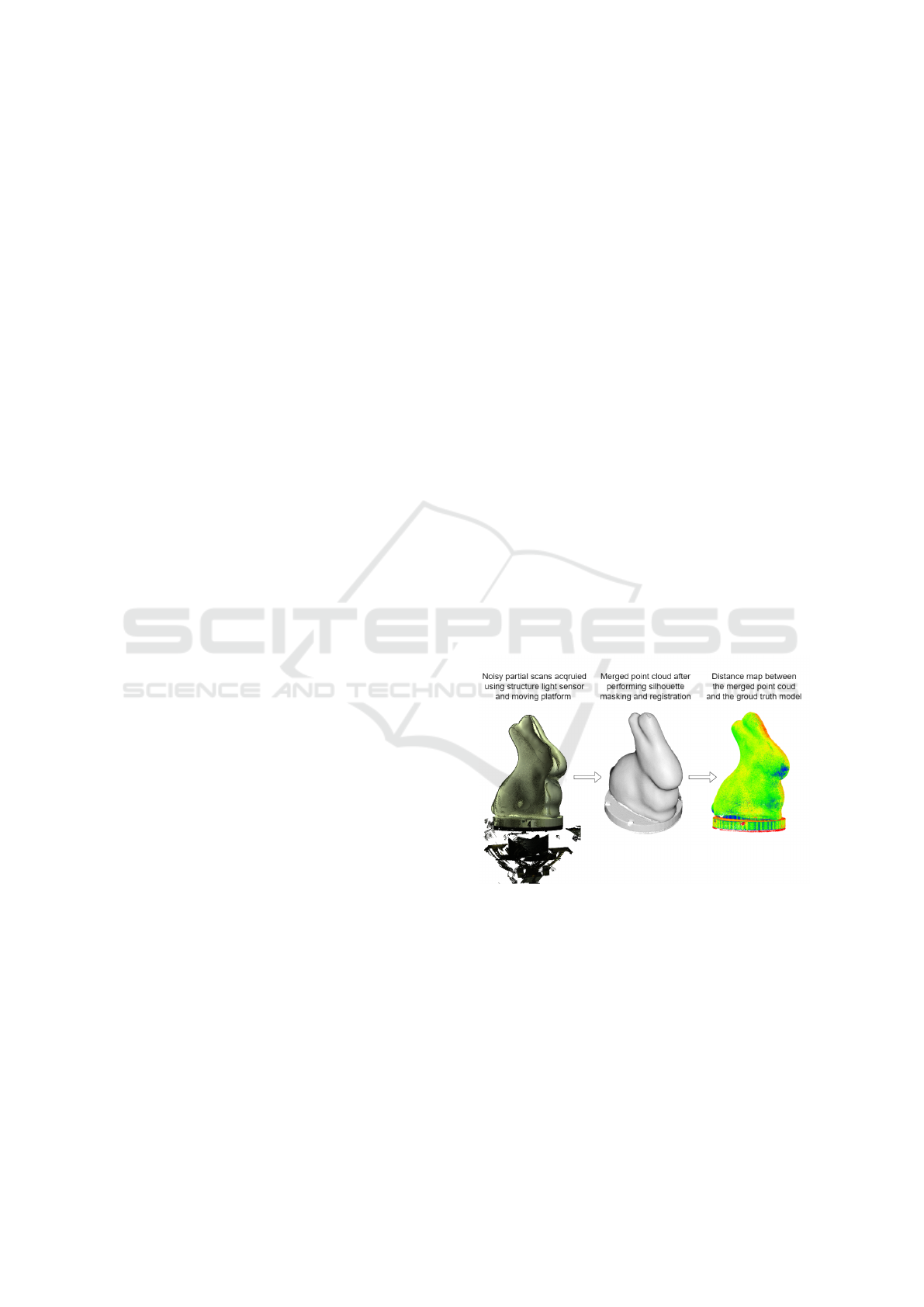
Figure 1: Overview of our point cloud measuring process.

First, we acquire partial scans that are aligned only via the

system calibration. Second, a ﬁltering process and a reﬁned

multi-point registration process leads to a merged point

cloud. Third, we measure the distance between our scanned

point cloud and the ground truth (e.g., CAD model).

ject, scanning from multiple viewpoints is necessary,

where several partial point clouds are co-registered

and merged into one. The matching of partial point

clouds relies on an accurate co-registration between

partial point clouds. This issue can be addressed

through extrinsic calibration of the scanning setup to

reach a rough initial alignment, and the evaluation of

Alibekov, U., Staderini, V., Ramachandran, G., Schneider, P. and Antensteiner, D.

Evaluation of 3D Point Cloud Distances: A Comparative Study in Multi-Point Cloud Fusion Environments.

DOI: 10.5220/0012421300003660

Paper published under CC license (CC BY-NC-ND 4.0)

In Proceedings of the 19th International Joint Conference on Computer Vision, Imaging and Computer Graphics Theory and Applications (VISIGRAPP 2024) - Volume 4: VISAPP, pages

59-71

ISBN: 978-989-758-679-8; ISSN: 2184-4321

reﬁned registration routines such as Global ICP (Glira

et al., 2015) or Pose Graph-based approaches (Choi

et al., 2015). Point cloud registration determines op-

timal transformations for global alignment, through

non-learning- (Yang et al., 2015) and learning-based

(Aoki et al., 2019) methods. The former are usually

based on applying an iterative optimization algorithm

to compute the rigid geometric transformation, while

learning-based approaches compute the transforma-

tion by extracting geometric features of the point

clouds. Existing research has predominantly focused

on large-scale scenes (e.g., SLAM (Kim et al., 2018)

and 3D scene reconstruction (Wang et al., 2023)).

After co-registration, the merged point cloud is

compared to a ground truth to assess the dimensional

accuracy and defects of the manufactured part. The

ground truth may be a mesh or a point cloud (e.g.,

from a CAD model or a highly precise reference

measurement). The analysis involves computing dis-

tances between object regions of the merged point

cloud and the reference ground truth (i.e., Cloud-to-

cloud or Cloud-to-mesh comparison), as described by

Sun and colleagues(Sun et al., 2023). However, this

task presents a challenge due to the unstructured na-

ture of point clouds, which lack a predeﬁned order in

their data representation. While various methods for

Cloud-to-cloud Distance computation have been pro-

posed (Wu et al., 2021), a comprehensive analysis of

how these tools are affected by point cloud complex-

ity, noise, and cloud density is missing.

Our contributions encompass the following:

• Implementation of a comprehensive pipeline, in-

volving partial point clouds acquisition, merging,

and comparison to the object’s ground truth.

• Evaluation of several state-of-the-art point cloud

reﬁnement techniques under various transforma-

tions such as translation and rotation.

• Thorough evaluation of metrics for measuring

cloud-to-cloud and cloud-to-mesh distances in di-

verse scenarios, including complex objects, ob-

jects with holes, and varying point cloud density.

2 RELATED WORK

2.1 Data Acquisition

Point clouds are commonly acquired through laser-

based or camera-based methods. In laser-based ap-

proaches, a sensor emits a beam towards the object,

and by measuring the time it takes for the light to re-

turn, the distance and 3D location where the laser hit

the object is determined (Wandinger, 2005).

Camera-based methods involve identifying dis-

tinctive points on the object’s surface and establish-

ing their correspondences in different images. For

example, active pattern projection projects structured

light patterns onto the object’s surface (Thorstensen

et al., 2021), deforming based on the object’s geome-

try. Captured by a camera, these patterns are then an-

alyzed. In stereo camera systems, two cameras with

a lateral separation (baseline) compute disparities be-

tween corresponding points in the two images, creat-

ing a 3D point cloud (Lee and Kweon, 2000). Multi-

view reconstruction integrates information from mul-

tiple 2D images, triangulating 3D positions for feature

matching across images, forming a point cloud (Seitz

et al., 2006).

2.2 Multi-Point Cloud Registration

2.2.1 Initial Alignment

In our real-world setup, the initial alignment of partial

point clouds relies on a well-calibrated scanning sys-

tem. In a robotic inspection setup, the end effector’s

position, carrying either the camera or the part to be

inspected, is known during calibration (Lattanzi and

Miller, 2017). However, over time, positional errors

accumulate due to inaccuracies in the motion axes of

the scanning system.

2.2.2 Classical Registration Methods

Many point cloud registration methods draw inspira-

tion from the iterative closest points (ICP) algorithm

by (Besl and McKay, 1992) and (Chen and Medioni,

1991). The ICP algorithm aims to achieve opti-

mal alignment or co-registration of overlapping point

clouds through a rigid-body transformation. The

ICP-based algorithm’s general pipeline, introduced

by (Rusinkiewicz and Levoy, 2001), consists of ﬁve

key stages: (i) selecting a subset of points within the

overlap area between two point clouds, and (ii) de-

termining the corresponding subset in the other point

cloud using the selected points; (iii) rejecting false

correspondences and (iv) determining a set of corre-

spondences with an associated set of weights; and (v)

estimating the (rigid-body) transformation by mini-

mizing the weighted and squared distances between

corresponding point, followed by applying the esti-

mated transformation. Challenges with the standard

ICP approach include the need for a good initial-

ization (pre-registration of partial point clouds) and

convergence to a local minimum. Another challenge

poses the pairwise matching between multiple point

clouds without a ﬁnal overall adjustment step for the

VISAPP 2024 - 19th International Conference on Computer Vision Theory and Applications

resulting merged point cloud, which leads to an accu-

mulating offset error.

Our work, based on a variant of the ICP algorithm

proposed by (Glira et al., 2015), focuses on match-

ing multiple point clouds (contrary to only pairwise

matching). Employing the original ICP algorithm

for matching points using k-d trees, the Global ICP

method introduces variations in strategies for select-

ing points in one point cloud (e.g. random or uni-

form sampling). Notably, Global ICP enables multi-

point cloud matching with a bundle adjustment step,

removing low-conﬁdence correspondences based on

point distances or surface normal orientations. The

transformation parameters are estimated by minimiz-

ing the sum of the squared distances between cor-

respondences, applying a rigid afﬁne transformation

(translation, rotation) to transform the point clouds.

By utilizing a single least squares optimization, it en-

sures that error propagation is handled correctly. Un-

like the traditional ICP, the proposed method works

well with large dataset, although, like any ICP-based

method, it depends on a good initial alignment.

Considered as an alternative, the pose Graph-

based approach proposed by (Choi et al., 2015) in-

volves creating a fully automatic geometric indoor

scene reconstruction pipeline from RGB-D video.

These scene fragments are connected into pose graph

where pose represent individual scene and edge con-

nects two nodes that overlap. The method registers

pairs of local scene fragments, constructing a global

model based on these alignments, with removal of

low-conﬁdence pairs based on the point cloud den-

sity. Subsequently, ICP is applied for reﬁnement, and

Pose Graph estimation yields the ﬁnal global frag-

ment pose.

2.2.3 Learning-Based Registration Methods

A review of deep learning methods for point cloud

registration based on rigid transformations was con-

ducted by (Zhang et al., 2020). They noted that ex-

isting feature extraction methods are mostly adapted

from modules designed for tasks like point cloud clas-

siﬁcation or segmentation. Dedicated methods specif-

ically tailored for registration are underdeveloped.

A survey of non-rigid transformation and

learning-based point cloud registration methods

was conducted by (Monji-Azad et al., 2023).

These were categorized as correspondence-free or

correspondence-based methods. Correspondence-

free methods often grapple with differences in global

features between point sets, while correspondence-

based methods face challenges related to missing

correspondences.

Deep learning methods prove beneﬁcial in solv-

ing the coarse registration problem by ﬁnding a coarse

initial transformation between two point clouds. They

excel in learning robust and distinct point feature

representations, particularly advantageous in scenar-

ios involving repetitive or symmetric scene elements,

weak geometric features (e.g. ﬂat object), or low-

overlap scenarios (Sarode et al., 2019).

Deep learning methodology was not utilized in

our work due to the small transformations between

partial scans of a single object. Additionally, indus-

trial precision requirements favor traditional methods

(Brightman et al., 2023).

2.3 Cloud-to-Cloud Distance

Measurements

Point clouds function as representations of object sur-

faces, capturing spatial information. When com-

paring two point clouds, fundamental for evaluating

the dissimilarity or similarity, are distance measure-

ments. Cloud-to-cloud distance measurements can be

broadly categorized into two approaches: point-to-

point distance and point-to-plane distance.

2.3.1 Point-to-Point Distance

In the point-to-point distance approach, the Eu-

clidean distance between individual points in two

point clouds is computed. In this case, S

∈ R

×3

and

∈ R

×3

represent the two point sets, with k

, k

be-

ing the number of points of the respective clouds. In-

dividual points are shown as p

∈ S

, p

∈ S

, so that

, p

∈ R

. The distance between two points is cal-

culated as follows:

d(x, y) = |p

− p

. (1)

The nearest neighbour function D

between

point p

and set S

then can be formulated as:

, S

) = min

∈S

d(p

, p

). (2)

Based on these deﬁnitions, common metrics for

point cloud distance computation using the point-to-

point method include:

Chamfer Distance - This metric computes the aver-

age sum of the squared distances for each point p

∈ S

to its nearest neighbour p

∈ S

(Wu et al., 2021):

, S

) =

∑

∈S

, S

)

∑

∈S j

, S

)

(3)

Evaluation of 3D Point Cloud Distances: A Comparative Study in Multi-Point Cloud Fusion Environments

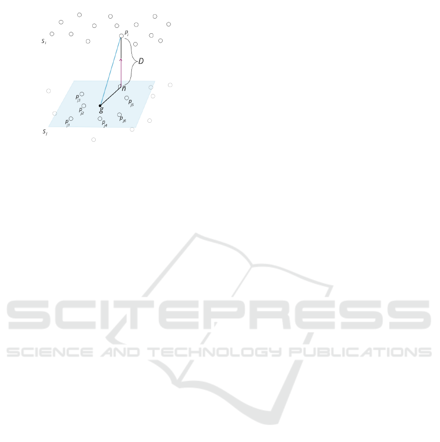
Figure 2: Visualization of the least squares distance be-

tween point p

and point cloud S

. The blue plane rep-

resents the best ﬁtting plane through the 6 nearest neigh-

bors p

, p

. The projection of the vector

from point p

and centroid g (mean value of nearest neigh-

bours) onto unit normal vector n depicts the distance D.

Hausdorff Distance - This metric calculates the max-

imum distance between any pair of nearest neigh-

bours between point clouds S

and S

(Huttenlocher

et al., 1993):

, S

) =

max



max

∈S

, S

), max

∈S

, S

)



. (4)

Earth Mover’s Distance - This is also known as the

Wasserstein distance. For each point p

in S

, it relates

a separate and distinct point in S

(bijection, ξ), so that

the sum of distances between corresponding points is

minimal (Yuan et al., 2018):

EMD

, S

) = min

ξ:S

→S

∑

∈S

− ξ(p

. (5)

Here, ξ represents a bijection. A function is bijec-

tive if, for every p

in S

, there exists exactly one p

such that ξ(p

) = p

(Koopman and Sportiche, 1982).

Both point clouds need the same number of points.

Computation of Earth Mover’s Distance (EMD) can

be quite resource-intensive and is typically used for

point clouds with a small to medium number of

points, typically around 5,000 or fewer (Fan et al.,

2017).

2.3.2 Point-to-Plane Distance

Another approach for computing the distance be-

tween two point clouds includes point-to-plane dis-

tance measurements. The distance from a point p

is calculated with respect to the best-ﬁtting plane

at S

, created through k-nearest neighbours (Peterson,

2009) or a speciﬁed search radius. A projection of

the vector between point p

and the centroid g (the

mean value of the nearest neighbours at S

) is com-

puted with respect to the unit normal vector n, which

represents the distance between p

and S

(see Figure

2).

By knowing that k represents the count of the

closest points p

, p

, ... p

to a given point p

, the

following distance measurements can be derived de-

pending on the ﬁtting function.

Least Squares Method - This method ﬁnds the least

squares best ﬁtting plane and computes the distance

from a point to that plane. The plane’s equation is

represented as follows:

x + λ

y + λ

= z. (6)

It is solved for the coefﬁcients λ

, λ

by using

a least squares method. The set of closest points

, p

, ... p

is represented as:

= x

Values for a, b and c are calculated that approximate

the system of equations to ﬁnd values for the follow-

ing equations:

+ λ

= z

+ λ

= z

+ λ

= z











This system of equations can be represented in matrix

format as:

Ax = b, (7)

where A, x and b are:

A =













, x =









, b =













The goal is to solve for the coefﬁcients of the best-

ﬁtting plane using least squares regression (Mu

noz

et al., 2014).

x =



· A



−1

· A

· b (8)

By solving for x, it is possible to obtain the coef-

ﬁcients λ

, λ

. Next, we need to compute the gra-

dient of the function, denoted as ∇ f , which is repre-

sented by a vector consisting of the partial derivatives

of the function with respect to the x, y, z axes.

∇ f =





∇ f





. (9)

VISAPP 2024 - 19th International Conference on Computer Vision Theory and Applications

By normalizing it, we can obtain the normal vector n

that is perpendicular to the surface:

n =

∇ f

|∇ f |

(10)

In the case of the Least squares method, the nor-

mal vector will be equal to the coefﬁcients λ

, λ

n =









(11)

As a result, the least squares distance from the point

to the plane can be computed using the cross product:

g · n|

|n|

= |p

g · n|, (12)

where p

g is the vector from the point p

to the cen-

troid g (mean value of all nearest neighbour points)

and n the unit normal vector.

Quadric - This method creates a quadratic best-ﬁtting

plane through the k closest points, and the distance is

calculated similarly to the Least squares method. The

function is given as follows:

+ λ

x + λ

xy + λ

y + λ

+ λ

= z (13)

Therefore, the system of equations of the plane pass-

ing through a set of the closest points p

, p

, ... p

will be:

+ λ

= z

+ λ

= z

···

+ λ

= z











By combining it into a matrix format similar to equa-

tion (7), it is possible to solve for x using the conju-

gate gradient optimization method (Nazareth, 2009).

This is an iterative optimization method starting with

an initial guess, where the solution is continuously re-

ﬁned by computing step sizes and search directions

and subsequently checked for convergence. As a re-

sult, the coefﬁcients λ

, λ

are de-

termined. Similar to equation (9), the gradient of the

function is calculated as follows:

∇ f =





∇ f









2λ

x + λ

+ λ

x + 2λ





(14)

By considering the centroid point g (mean value

of nearest neighbour points) and inserting the x, y, z

values into equation (14), the normal vector can be

computed using equation (10). Finally, the distance

can be computed similarly to equation (12) as quadric

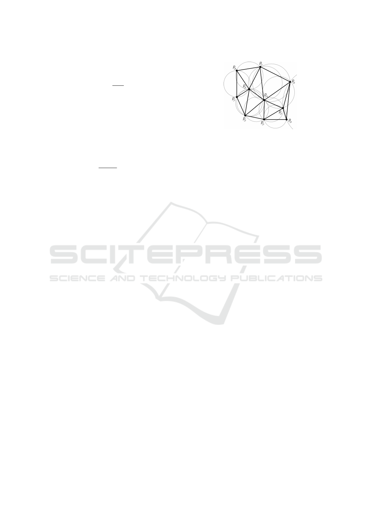
Figure 3: Visualization of the Delaunay triangulation for

ten points from a top view perspective. Each dot represents

a point of the point cloud. The Delaunay triangulation max-

imizes the minimum angle of all the angles of the triangles

so that no point is inside the circumcircle of any triangle.

2.5D Triangulation - In Delaunay triangula-

tion (Chen and Xu, 2004), the 2.5D means that the

points are projected onto best-ﬁtting plane and 2D

triangulation is performed in this plane. Afterwards,

the algorithm forms triangles, and creates a 2.5D

mesh. The distance between a point and the 2.5D

mesh is computed by ﬁnding the closest triangle (see

Figure 3) and performing a point-to-plane distance

computation.

The original 3D points are used as vertices for the

mesh to create a 2.5D mesh. The distance between

a point to the 2.5D mesh is computed by ﬁnding the

closest triangle to the point and performing a point-

to-plane distance computation. As a result, the 2.5D

triangulation D

T RI

distance can be computed.

2.4 Cloud-to-Mesh Distance

Measurement

A mesh is a collection of vertices, edges, and faces

that deﬁne the shape of a 3D object. Usually, the

faces of the mesh are composed of triangles (triangle

mesh), quadrilaterals (quads), or other simple convex

polygons (n-gons) (Cobb et al., 2009). The Cloud-

to-mesh Distance D

C2M

is found in a similar way as

in Sec. 2.3.2, where the plane is represented by the

triangle of the mesh. If the orthogonal projection of

the point on this plane is outside of the triangle, then

the distance to the nearest edge is taken. Taking into

account the orientation of the normal vector, the cal-

culated distance is signed, indicating that the point is

considered outside the mesh when the distance is pos-

itive and inside when it is negative.(Jones, 1995).

3 METHODOLOGY

In this section, we outline our methodology, encom-

passing data generation, point cloud registration, and

Evaluation of 3D Point Cloud Distances: A Comparative Study in Multi-Point Cloud Fusion Environments

evaluation using various distance metrics.

To this end, we performed experiments on three

types of data: (i) we synthetically generated point

clouds with well-deﬁned shapes (e.g., plane, slope,

sine wave, and triangular wave); (ii) simulated point

cloud acquisitions using ray tracing with a 3D mesh

of an object with a CAD model; and (iii) point clouds

obtained experimentally using a structured light sen-

sor and a precise kinematic setup.

Accurate point cloud registration was achieved by

an initial alignment step and further calibration and

reﬁnement steps. Additionally, we present our evalu-

ation process involving diverse distance metrics.

3.1 Synthetic Data Generation of

Well-Deﬁned Shapes

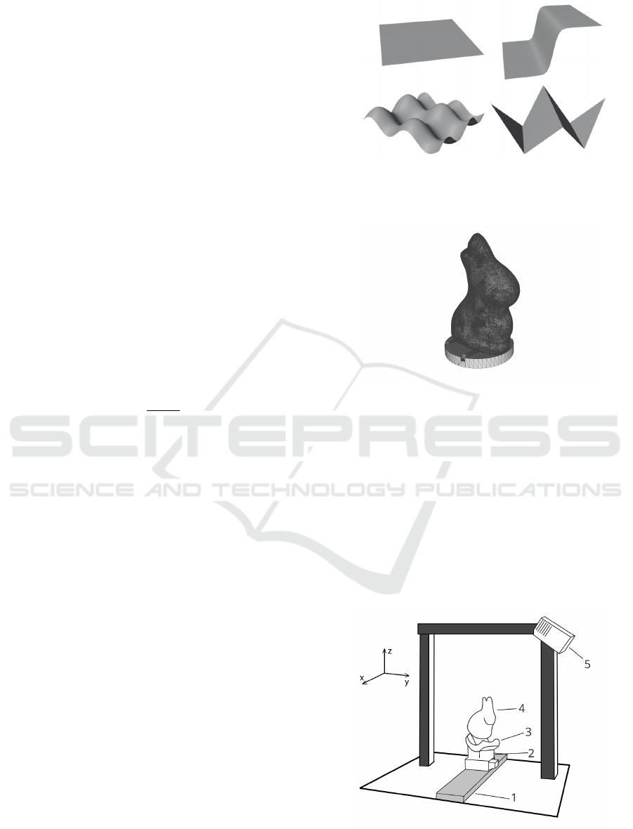
We generated meshes for four distinct shapes: plane,

slope, sinusoidal wave, and triangular wave. These

meshes represent different degrees of shape complex-

ity. The surface equations used in Blender are shown

in the following.

Plane: z = 0

Slope: z =

1 + ε

Sine wave: z = sin(2πx) + sin(2πy)

Triangular wave: z =

mod (x + y, 2) − 1

− 0.5

The shapes were subdivided into 16 segments or parts

along each axis. The subdivision tool of Blender al-

lows one to break down a bigger object into smaller

components creating a detailed mesh. Each object has

dimensions of 1 meter in both width and length, mak-

ing it comparable to real-world data in terms of size.

The generated meshes are displayed in the Figure 4.

3.2 Synthetic Data Generation of

Partial Scans

We utilized the 3D mesh of a rabbit (see Figure 5) to

synthesize a sensor capturing the object from various

viewpoints. To ensure comprehensive object cover-

age, we employed the method proposed in (Staderini

et al., 2023) based on Poisson disc sampling to deter-

mine optimal camera poses in terms of coverage. This

method was chosen for its simplicity of implementa-

tion and its ability to achieve extensive coverage with

only a small number of optimal views. To capture par-

tial scans of the object under inspection, we employed

ray tracing. The sensor model used had a resolution

of 1920 × 1200 pixels, a ﬁeld of view (FOV) spanning

Figure 4: Different meshes used in this work (plane, slope,

sine wave, triangular wave). Each mesh shows a different

degree of shape complexity. The shapes from the top view

are squares. The meshes have been generated in Blender.

Figure 5: 3D mesh of the inspected object. This model was

adopted in our simulation and was used to 3D-print the ob-

ject on which real-world experiments (i.e., scanning) in the

lab were conducted.

38.70

◦

× 24.75

◦

, and a depth of ﬁeld (DOF) between

350mm and 700 mm, ensuring consistency with the

parameters used in acquiring the experimental data in

the lab.

The synthetically generated (and therefore

aligned) partial scans were rigidly transformed to

establish ground truth transformations. This informa-

tion can later be used for the evaluation of registration

methods, where the estimated transformation matrix

is compared against the ground truth transformation.

Figure 6: Schematics of the hardware lab setup. 1 - moving

linear stage, 2 - rotating stage, 3 - tilt stage (goniometer), 4

- object that is being scanned, 5 - structured light sensor.

VISAPP 2024 - 19th International Conference on Computer Vision Theory and Applications

3.3 Experimental Data Acquisition

For real-world point cloud acquisition in the lab, we

utilized a Zivid One+ S structured light sensor, to con-

duct experiments with a 3D-printed rabbit (Figure 5),

which matched the 3D mesh used in our simulations.

The model of the 3D printer is Stratasys F370 with

0.2 mm accuracy. We evaluated the Cloud-to-cloud

Distance metrics on our real-world point cloud acqui-

sitions. The camera-object poses were determined ac-

cording to the optimal viewpoint generation method

described in (Staderini et al., 2023). Our camera re-

mained stationary while the object had three degrees

of freedom on a precise kinematic setup involving a

linear axis, a rotary table, and a goniometer (see Fig-

ure 6). The moving linear stage moves in x-direction,

whereas the rotating stage and the goniometer enable

rotations along all spatial directions.

With our kinematic setup, we achieve a high ac-

quisition accuracy. On this account, we could use

the joint values of the kinematic setup and the extrin-

sic parameters of the camera to obtain a good initial

alignment of the acquired point clouds. Additionally,

we applied a pre-processing step to reduce outliers

and noise, where silhouette masking was employed

as described in (Rousseeuw, 1987). The ground truth

mesh model was positioned at the actual location of

the object, and points were removed, which were far-

ther away from the model than a certain threshold.

Afterwards, the point cloud density was computed.

Low-density regions were identiﬁed as noise and re-

moved.

3.4 Point Cloud Registration

3.4.1 Initial Alignment

For lab data acquisition, our experimental setup com-

prised a kinematic chain with a linear stage mov-

ing a rotating stage, with a tilt stage (see Figure

6). Multiple partial acquisitions from various view-

ing angles generated the point clouds. These partial

point clouds were co-registered, with the initial align-

ment achieved through forward kinematics utilizing

the three actuators. The initial joint positions were

saved, and for each joint, the travel between the cur-

rent and initial positions was calculated. Adjustments

to the rotating stage axis and tilt stage were made ac-

cordingly. To address orientation misalignment, the

object underwent rotations along the new tilt and ro-

tating stage axes. Correcting positional misalignment

caused by the linear stage movement involved trans-

lating the object along the linear stage axis in the in-

verse travel direction. The subsequent step involves

the reﬁned registration of the partial point clouds.

(a) (b) (c)

Figure 7: Examples of a triangular wave with different

imperfections: (a) density/sparsity (with a deﬁned den-

sity/sparsity level), (b) noise (with a deﬁned standard de-

viation) and (c) hole (with a deﬁned radius).

3.4.2 Reﬁned Registration

We assessed the Global ICP and Pose Graph regis-

tration methods detailed in Sec. 2.2 using synthetic

data (see Sec. 3.2). After generating partial scans

from various viewpoints, initially six, then expanding

to ten, we systematically applied random transforma-

tions such as translation and rotation to them in order

to assess the registration performance.

3.5 Evaluation Using Distance Metrics

We evaluated various distance metrics, including

Chamfer, Hausdorff, Least Squares, Quadric, 2.5D

Triangulation and Cloud-to-Mesh. The Earth Mover’s

Distance was excluded due to its requirement of point

clouds with identical numbers of points.

Meshes (see Figure 4) were uniformly sampled

with 1000 points, and a cloned point cloud was shifted

above the original along the z-axis by 0.5 units (/me-

ters). Varied conditions, including sampling factor,

noise, and the introduction of a hole were applied to

this shifted point cloud.

The linear sampling number was set to vary the

shifted point cloud’s density from 0 to 1, where 0 rep-

resents the same density as the original point cloud,

and 1 indicates no points. The sampling number de-

cresed by 100 points at each 0.1 step. We introduced

normally distributed noise with a varying standard de-

viation (0.01 to 0.1 units, mean value of 0) and created

a hole by removing points within a circle centered at

the shifted point cloud’s centroid, with a radius vary-

ing from 0.1 to 1 units.

4 RESULTS

4.1 Comparison of Different

Registration Methods

We assessed registration methods using synthetic par-

tial scans (as detailed in Sec. 3.2) acquired from vary-

ing numbers of viewpoints, simulating our lab setup

Evaluation of 3D Point Cloud Distances: A Comparative Study in Multi-Point Cloud Fusion Environments

Average translation

Average rotation

(a) Global ICP.

Average translation

Average rotation

(b) Pose Graph.

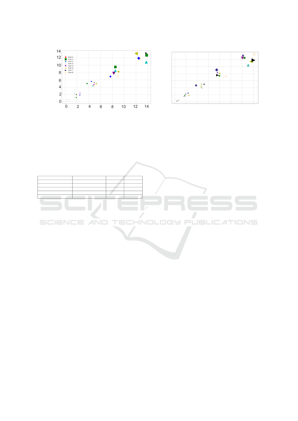
Figure 8: Evaluation of Global ICP and Pose Graph in terms of randomly applied rotations and translations to the partial scans

obtained from eight different viewpoints. Each coloured icon represents one partial scan. The size of the icon represents the

absolute mean error.

Table 1: Average absolute mean errors across eight point

cloud scans for Global ICP and Pose Graph registration

methods. The different conﬁgurations of point cloud scans

were retrieved based on arbitrary rotation and translation er-

rors in the ranges indicated in the table.

Rotation range (degrees) Translation range (mm) Global ICP Pose Graph

[0,1] [0,1] 0.0045 0.0352

[1,3] [1,3] 0.0416 0.0567

[3,6] [3,6] 0.1668 0.1718

[6,10] [6,10] 0.5482 0.5117

[10,15] [10,15] 0.5280 0.5789

shown in Figure 6. Random rotational and transla-

tional transformations (0 to 15 degrees and 0 to 15

mm) were applied. Global ICP and Pose Graph meth-

ods (described in Sec. 2.2) were used to register these

partial scans and the absolute mean error between

ground truth transformation and estimated transfor-

mation were computed as shown in Figure 8a and

Figure 8b. The quantitative representation of the re-

sults is shown in Table 1.

In Figure 8b coloured icons represent differ-

ent partial scans from various viewpoints, with the

icon size indicating absolute mean error magnitude.

Notably, registration was conducted relative to the

ﬁrst scan, leading to zero error due to the applied

transformation being the identity matrix. For small

transformations (see Figure 8) both methods aligned

point clouds well, but Global ICP outperformed Pose

Graph. Numeric results are shown in Table 1. Due

to time constrains, the test was randomly performed

once, possibly explaining Pose Graph’s occasional

better accuracy. However, as we expanded the applied

transformations range from 0 to 15 (Figure 8), abso-

lute mean error for both methods increased. In our ex-

periments, Pose Graph sensitivity to parameters like

voxel size, maximum correspondence distance, and

edge pruning threshold resulted in higher error. Con-

sequently, the Global ICP registration method was

chosen.

4.2 Comparison of Different

Cloud-to-Cloud Distance Methods

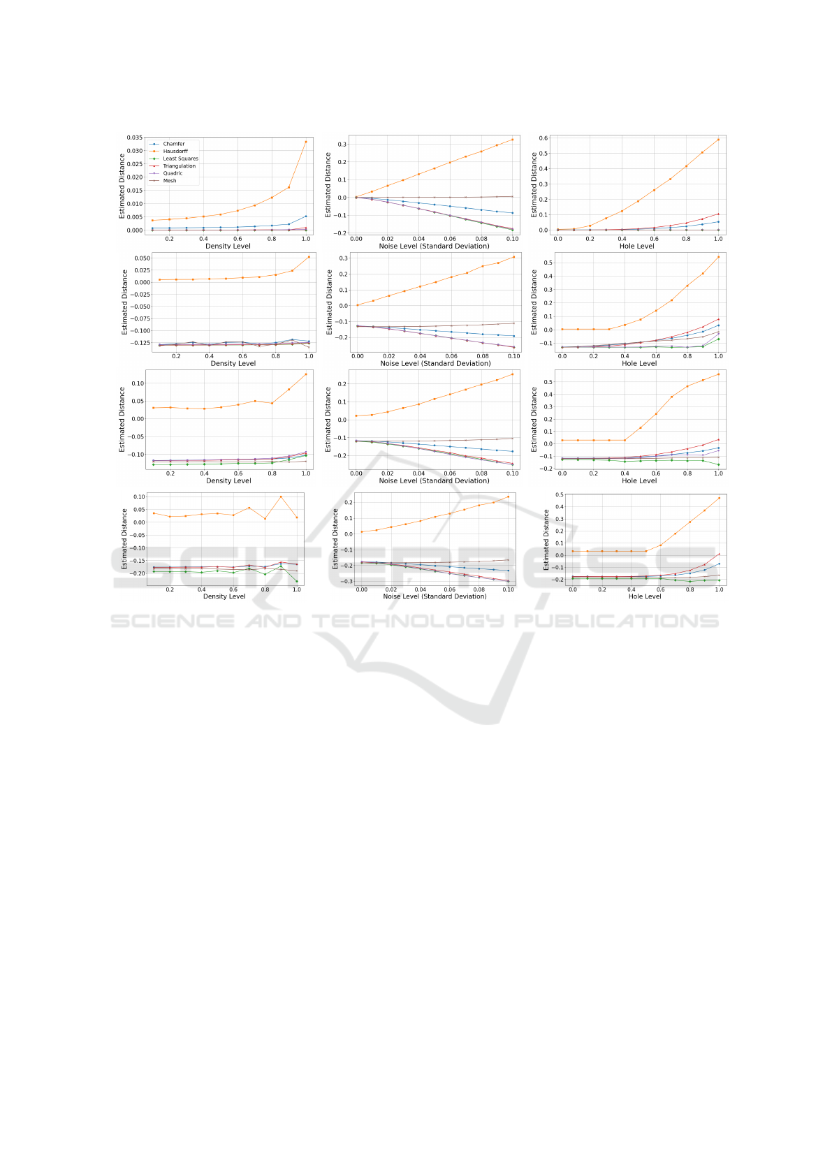
Various distance metrics were assessed with respect

to point density, noise level, and hole radius, as shown

in Figure 9. The y-axis represents the deviation from

the ground truth distance, while the x-axis illustrates

different levels of point density, noise, and hole ra-

dius. To ensure unbiased results, each plot has been

obtained by computing an average value, calculated

from 100 executions. The implementation of the dis-

tance measurements was based on a Python wrapper

for CloudCompare called CloudComPy (Girardeau-

Montaut, 2016).

Upon reviewing the results following insights

emerge:

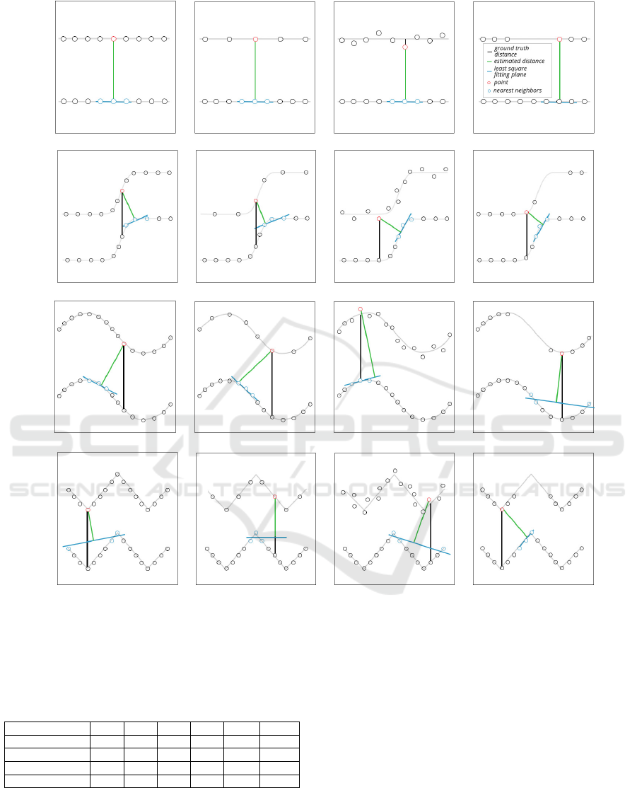
• The shapes of objects play a crucial role in in-

ﬂuencing the outcomes for different point cloud

distance metrics. This stems from the fact that

the methods rely on nearest neighbour searches,

where complex shapes can lead to incorrect

matches. For example, in Figure 10 we can ob-

serve that depending on the shape of a surface,

the Least squares method struggles to ﬁnd the cor-

rect distance between planes. In the case of a

slope, points on the inclined part of the shape’s

surface are incorrectly associated with the clos-

est points on the reference surface, resulting in

distance measures that are underestimated. More-

over, for the triangular wave, the closest points to

the tip of the triangle are distributed on both sides

of the wave, leading to a inadequate ﬁtting line

and inaccurate distance estimations.

• The Hausdorff Distance, calculated by determin-

ing the maximum distance between any pair of

nearest neighbours, provides the best results for

VISAPP 2024 - 19th International Conference on Computer Vision Theory and Applications

PlaneSlope

Sine wave

Triangular Wave

Density Noise Hole

Figure 9: Evaluation of the distance metrics on a plane, slope, sine wave, and triangular wave shape. Each result is an average

after 100 executions. The distance is given with respect to the ground truth distance (a perfect result would have an estimated

distance of 0.0), with increasing levels of density, noise, and size of the hole in the point clouds.

all shapes when the point cloud is free of per-

turbations. Its sensitivity becomes noticeable as

the levels of noise, density variations, and size

of the hole increase, diverging considerably from

other distance metrics. The introduction of pertur-

bations increases the maximum distance between

pairs of nearest neighbours, leading to poor esti-

mation of the distance between point cloud and

the ground truth. This behaviour was later con-

ﬁrmed when testing with real life objects (see Ta-

ble 3).

• The Chamfer Distance demonstrates comparable

accuracy to point-to-plane distance metrics, ex-

cept in the context of varying levels of noise. Un-

like other methods, the Chamfer Distance is less

affected by noise. This can be explained by the

fact that the Chamfer Distance is based on averag-

ing, which acts as a mitigating factor against the

impact of noise.

• It was found that the changing point cloud den-

sity and hole size (see Figure 7) does not signif-

icantly affect the distance estimation. However,

when increasing the hole radius for slope, sine

wave, and triangular wave shapes, the distance es-

timation is getting closer to the correct value. This

can be explained by the fact that with a decreasing

inﬂuence of the surface complexity, more points

in the middle of the mesh are being removed. On

the other hand, increasing the radius of the hole

for the plane shape decreases the estimated dis-

tance accuracy, because individual points are far-

ther away from each other.

• The Cloud-to-mesh Distance measurement pro-

vided the best results when the noise, hole, and

density levels are high (see Table 2). We be-

lieve that small error changes with respect to the

added noise result from the uniform distribution

of the applied noise. When computing the dis-

tance, the averaging step neutralizes the effect of

Evaluation of 3D Point Cloud Distances: A Comparative Study in Multi-Point Cloud Fusion Environments

PlaneSlope

Sinewave

Triangular Wave

Original Density Noise Hole

Figure 10: Illustration of the Least squares distance metric for the synthetically generated shapes (plane, slope, sine wave,

triangular wave). Our different varitions/conditions (point cloud density, noise, hole) have been applied as shown in the ﬁgure.

The corresponding rendered shapes are shown in Figure 4.

Table 2: Evaluation of distance metrics on synthetic data

with average levels of noise (0.07), hole (0.5) and point den-

sity (0.4).

T RI

C2M

Plane 0.40 0.21 0.11 0.12 0.10 0.01

Slope 0.25 0.27 0.19 0.18 0.16 0.09

Sine wave 0.22 0.20 0.19 0.18 0.17 0.12

Triangular wave 0.12 0.11 0.22 0.22 0.21 0.18

the noise. Furthermore, point-to-point and point-

to-plane distance methods depend on a nearest

neighbor search, which yields a signiﬁcant sen-

sitivity to noise.

4.3 Comparison with Ground Truth

Model

After applying the registration step to the partial

scans, a merged point cloud was created (see Fig-

ure 1). To correctly analyze the results, compar-

ing it to a ground truth model is essential. For the

Cloud-to-cloud Distance the reference model (e.g.,

CAD model) was sampled to a point cloud. For the

Cloud-to-mesh Distance, the ground truth mesh of

the reference model was used directly to compute the

distance. The results were visualized using Cloud-

Compare v.2.13.alpha software (Girardeau-Montaut,

VISAPP 2024 - 19th International Conference on Computer Vision Theory and Applications

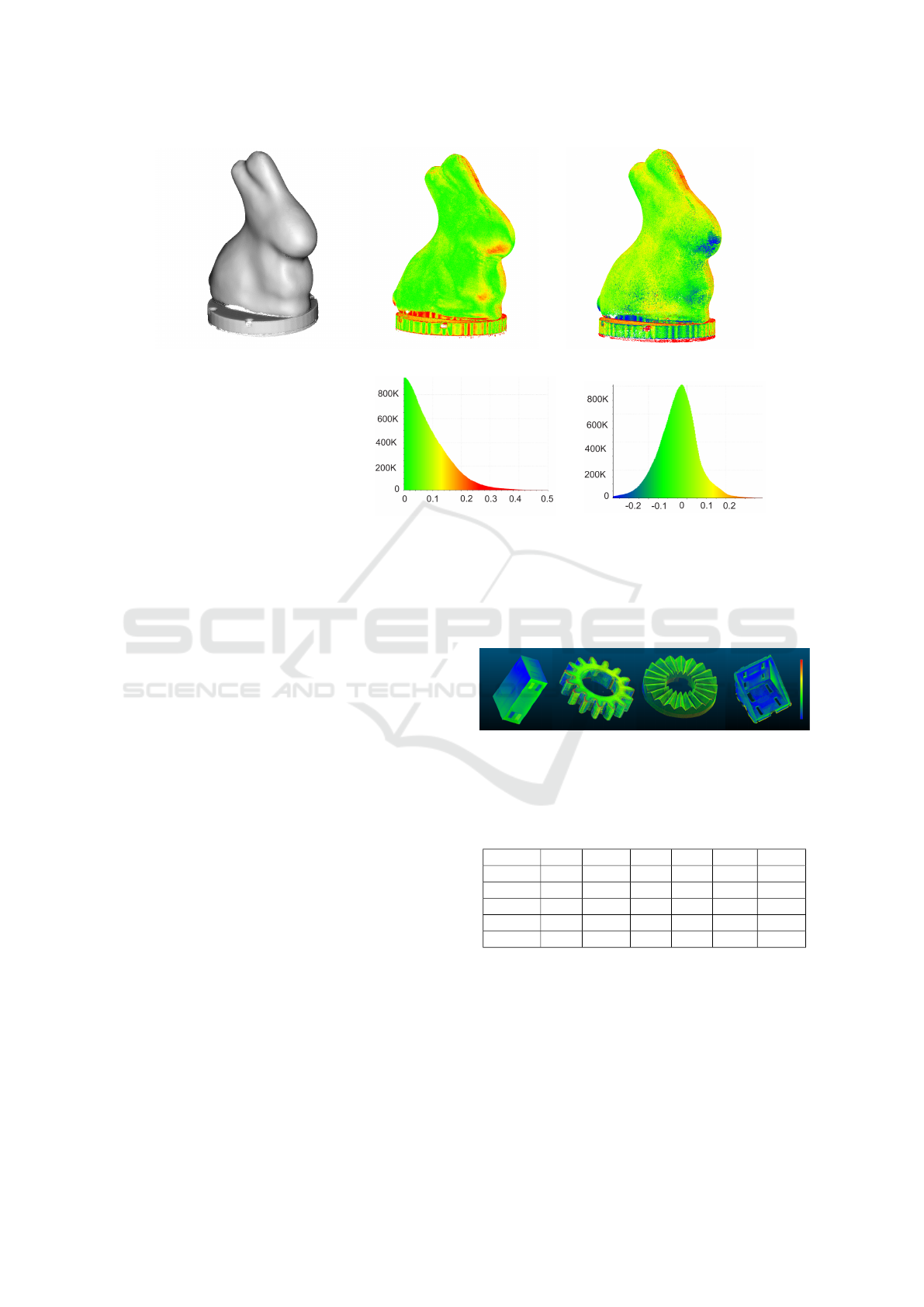
Merged point cloud. Cloud-to-cloud method. Cloud-to-mesh method.

C2C distance

Count

C2M signed distance

Count

Figure 11: Illustration of the distribution of distances using two different distance metrics. On the left, the merged point

cloud is shown after silhouette masking on partial scans and performing Global ICP registration. On this merged point cloud

we visualize the distribution of distances compared to the ground truth point cloud using the Least squares Cloud-to-cloud

Distance (centre) and Cloud-to-mesh Distance (right). The histograms of distances obtained by the Least square Cloud-to-

cloud or C2C Distance and the Cloud-to-mesh or C2M signed Distance are shown at the bottom center and right, respectively.

2016).

Comparison with Point Cloud. As detailed in

Sec. 2.3, various methods for computing Cloud-to-

cloud Distance exist. However, some of the distance

metrics cannot be used in our case. For instance, the

Earth Mover’s Distance requires both the reference

and compared point cloud to have the same number

of points, which is not possible in our experiments.

Additionally, Chamfer and Hausdorff Distances pro-

vide only one value as a distance metric, while for in-

dustrially relevant scenarios, it would be beneﬁcial to

retrieve the distribution of distances across the entire

point cloud, in order to detect any imperfections due

to manufacturing problems for instance. However, for

evaluation purposes both methods were also included

in the Table 3. The point-to-plane methods exhibited

similar results (see Figure 9 ). However, in our real-

life testing based on lab acquisitions, the plane ﬁtting

method demonstrated more accurate estimation of the

distance compared to the rest Cloud-to-cloud methods

(see in Table 3).

Comparison with Mesh. The merged point cloud

can be directly compared to the 3D mesh (shown in

Figure 5). The computation involves determining the

distance between individual points of the combined

point cloud and the nearest triangle of the mesh. The

Figure 12: The distance map for cube, gear, hirt and bracket

objects (from left to right). Colors represent the points’ de-

viation from ground truth, ranging from red (higher error)

to blue (lower error) with yellow and green color between.

Table 3: Evaluation of Distance metrics on different real

world data, objects shown in Figure 12.

T RI

C2M

bunny 0.18 9.97 0.08 0.09 0.13 0.03

hirt 1.06 13.74 0.14 0.16 0.16 0.03

cube 1.76 48.98 0.49 0.53 0.54 0.42

gear 0.43 9.66 0.16 0.18 0.19 0.05

bracket 0.94 9.56 0.72 0.74 0.74 0.28

resulting distances have signed values based on the

orientation of the triangle normal.

To objectively test the distance metrics in real life

scenario, ﬁve objects with various complexities were

chosen (see Figure 11 and Figure 12). It was exper-

imentally observed that the Cloud-to-mesh method

provide better estimation of the distance. The abso-

lute mean value for the Cloud-to-mesh was found to

be lower across all scenarios. The distribution of the

Evaluation of 3D Point Cloud Distances: A Comparative Study in Multi-Point Cloud Fusion Environments

distances as histogram for Cloud-to-mesh and Least

Squares methods can be seen on Figure 11.

5 CONCLUSIONS

In this paper, we conducted a comprehensive evalu-

ation of 3D point cloud distances, focusing on their

performance in multi-point cloud fusion scenarios.

Our evaluation involved synthetic partial scans gen-

erated under various viewpoints. Misalignment errors

were synthetically introduced through random rota-

tional and translational transformations. The compar-

ison of Global ICP and Pose Graph methods showed

that while both methods show a lower accuracy as

the degree of the applied transformations increase,

Global ICP showed to perform better under small

synthetic transformation (translation, rotation) errors.

Pose Graph showed to be more sensitive to initial pa-

rameter settings such as voxel size, maximum corre-

spondence distance, and edge pruning threshold.

Our investigation into Cloud-to-cloud Distance

metrics revealed shape-dependent accuracy varia-

tions. As the complexity of the shapes increased, the

nearest neighbours search, which is the core of all

methods, led to incorrect generation of correspond-

ing points. In the case of the slope, points on the in-

clined part of the shape’s surface were mistakenly as-

sociated with the nearest points on the reference sur-

face. This led to underestimated distance measure-

ments (See Figure 10). The Hausdorff Distance ex-

hibited sensitivity to perturbations, while the Cham-

fer Distance demonstrated resilience to noise due to

its averaging mechanism. Changes in point cloud

density and hole levels had negligible effects on the

distance measurements. Notably, the Cloud-to-mesh

Distance computation consistently provided superior

results across different perturbations and shapes.

In the context of real-world industrial scanning,

our approach involved an initial alignment through

the calibration of the kinematic system used for scan-

ning, and a pre-processing step to remove sensor-

induced background noise. This was done using sil-

houette masking to reduce noise and applying the

Global ICP registration to merge the partial scans.

Cloud-to-cloud and Cloud-to-mesh Distance metrics

were introduced to evaluate the merged point cloud

obtained from ﬁve different objects. By looking at the

Table 3, it can be seen that Cloud-to-mesh Distance

provided better distance estimation compared to the

rest of the methods.

Future work will focus on reﬁning registration

methods tailored to address the challenges of complex

industrial scanning scenarios. Furthermore, enhance-

ments to distance metrics for varying point densi-

ties, noise levels, and geometric complexities will be

pursued. Improvement suggestions include increas-

ing the number of nearest neighbours to reach an im-

proved surface approximation and adding texture pri-

ors. Real-world materials can show transparencies,

dark areas, and highly reﬂective regions. Addition-

ally, the use of texture priors shall be explored for in-

dustrial object evaluation and measurement that are

highly accurate.

REFERENCES

Aoki, Y., Goforth, H., Srivatsan, R. A., and Lucey, S.

(2019). Pointnetlk: Robust & efﬁcient point cloud reg-

istration using pointnet. In CVPR, pages 7163–7172.

Besl, P. and McKay, N. D. (1992). A method for registration

of 3-d shapes. IEEE Transactions on Pattern Analysis

and Machine Intelligence, 14(2):239–256.

Brightman, N., Fan, L., and Zhao, Y. (2023). Point cloud

registration: A mini-review of current state, challeng-

ing issues and future directions. AIMS Geosci, 9:68–

85.

Chen, L. and Xu, J.-c. (2004). Optimal delaunay triangula-

tions. Journal of Computational Mathematics, pages

299–308.

Chen, Y. and Medioni, G. (1991). Object modeling by reg-

istration of multiple range images. In Proceedings.

1991 IEEE International Conference on Robotics and

Automation, pages 2724–2729 vol.3.

Choi, S., Zhou, Q.-Y., and Koltun, V. (2015). Robust re-

construction of indoor scenes. In CVPR, pages 5556–

5565.

Cobb, W., Peindl, R., Zerey, M., Carbonell, A., and Heni-

ford, B. (2009). Mesh terminology 101. Hernia, 13:1–

Fan, H., Su, H., and Guibas, L. J. (2017). A point set gen-

eration network for 3d object reconstruction from a

single image. In CVPR, pages 605–613.

Girardeau-Montaut, D. (2016). Cloudcompare. France:

EDF R&D Telecom ParisTech, 11.

Glira, P., Pfeifer, N., Briese, C., and Ressl, C. (2015).

A correspondence framework for als strip ad-

justments based on variants of the icp algorithm.

Photogrammetrie-Fernerkundung-Geoinformation,

2015(4):275–289.

Huo, L., Liu, Y., Yang, Y., Zhuang, Z., and Sun, M. (2023).

Research on product surface quality inspection tech-

nology based on 3d point cloud. Advances in Mechan-

ical Engineering, 15(3):16878132231159523.

Huttenlocher, D. P., Klanderman, G. A., and Rucklidge,

W. J. (1993). Comparing images using the hausdorff

distance. IEEE TPAMI, 15(9):850–863.

Jones, M. W. (1995). 3d distance from a point to a triangle.

Department of Computer Science, University of Wales

Swansea Technical Report CSR-5, page 5.

VISAPP 2024 - 19th International Conference on Computer Vision Theory and Applications

Kim, P., Chen, J., and Cho, Y. K. (2018). Slam-driven

robotic mapping and registration of 3d point clouds.

Automation in Construction, 89:38–48.

Koopman, H. and Sportiche, D. (1982). Variables and the

bijection principle.

Lattanzi, D. and Miller, G. (2017). Review of robotic infras-

tructure inspection systems. Journal of Infrastructure

Systems, 23(3):04017004.

Lee, D. and Kweon, I. (2000). A novel stereo camera sys-

tem by a biprism. Transactions on Robotics and Au-

tomation (T-RO), 16(5):528–541.

Monji-Azad, S., Hesser, J., and L

ow, N. (2023). A review of

non-rigid transformations and learning-based 3d point

cloud registration methods. ISPRS Journal of Pho-

togrammetry and Remote Sensing, 196:58–72.

noz, L. R., Villanueva, M. G., and Su

arez, C. G. (2014).

A tutorial on the total least squares method for ﬁtting

a straight line and a plane. Revista de Ciencia e Ingen.

del Institute of Technology, Superior de Coatzacoal-

cos, 1:167–173.

Nazareth, J. L. (2009). Conjugate gradient method. Wiley

Interdisciplinary Reviews: Computational Statistics,

1(3):348–353.

Peterson, L. E. (2009). K-nearest neighbor. Scholarpedia,

4(2):1883.

Rousseeuw, P. J. (1987). Silhouettes: a graphical aid to

the interpretation and validation of cluster analysis.

Journal of computational and applied mathematics,

20:53–65.

Rusinkiewicz, S. and Levoy, M. (2001). Efﬁcient variants

of the icp algorithm. In Proceedings Third Interna-

tional Conference on 3d Digital Imaging and Model-

ing, pages 145–152.

Sarode, V., Li, X., Goforth, H., Aoki, Y., Srivatsan,

R. A., Lucey, S., and Choset, H. (2019). Pcr-

net: Point cloud registration network using pointnet.

arXiv:1908.07906.

Seitz, S. M., Curless, B., Diebel, J., Scharstein, D., and

Szeliski, R. (2006). A comparison and evaluation

of multi-view stereo reconstruction algorithms. In

CVPR, volume 1, pages 519–528. IEEE.

Staderini, V., Gl

uck, T., Schneider, P., Mecca, R., and Kugi,

A. (2023). Surface sampling for optimal viewpoint

generation. In ICPRS, pages 1–7. IEEE.

Su, S., Wang, C., Chen, K., Zhang, J., and Yang, H. (2021).

Mpcr-net: Multiple partial point clouds registration

network using a global template. Applied Sciences,

11(22).

Sun, W., Wang, J., Yang, Y., Jin, F., and Sun, F. (2023).

Accurate deformation analysis based on point posi-

tion uncertainty estimation and adaptive projection

point cloud comparison. Geocarto International, page

2175916.

Thorstensen, J., Thielemann, J. T., Risholm, P., Gjessing,

J., Dahl-Hansen, R., and Tschudi, J. (2021). High-

quality dense 3d point clouds with active stereo and a

miniaturizable interferometric pattern projector. Op-

tics Express, 29(25):41081–41097.

Wandinger, U. (2005). Introduction to lidar. In Lidar:

range-resolved optical remote sensing of the atmo-

sphere, pages 1–18. Springer.

Wang, H., Liu, Y., Dong, Z., Guo, Y., Liu, Y.-S., Wang, W.,

and Yang, B. (2023). Robust multiview point cloud

registration with reliable pose graph initialization and

history reweighting. In CVPR.

Wu, T., Pan, L., Zhang, J., Wang, T., Liu, Z., and Lin,

D. (2021). Density-aware chamfer distance as a

comprehensive metric for point cloud completion.

arXiv:2111.12702.

Yang, J., Li, H., Campbell, D., and Jia, Y. (2015). Go-

icp: A globally optimal solution to 3d icp point-set

registration. IEEE TPAMI, 38(11):2241–2254.

Yuan, W., Khot, T., Held, D., Mertz, C., and Hebert, M.

(2018). Pcn: Point completion network. In Interna-

tional conference on 3d vision (3DV), pages 728–737.

IEEE.

Zhang, Z., Dai, Y., and Sun, J. (2020). Deep learning based

point cloud registration: an overview. Virtual Real-

ity & Intelligent Hardware, 2(3):222–246. 3d Visual

Processing and Reconstruction Special Issue.

Evaluation of 3D Point Cloud Distances: A Comparative Study in Multi-Point Cloud Fusion Environments