Biologically-Informed Shallow Classification Learning Integrating
Pathway Knowledge
Julius Voigt
1 a
, Sascha Saralajew
2 b
, Marika Kaden
1 c
, Katrin Sophie Bohnsack
1,3 d
,
Lynn Reuss
1 e
and Thomas Villmann
1 f
1
Saxon Institute for Computational Intelligence and Machine Learning,
University of Applied Sciences Mittweida, Mittweida, Germany
2
NEC Laboratories Europe GmbH, Heidelberg, Germany
3
Bernoulli Institute for Mathematics, Computer Science and Artificial Intelligence,
University of Groningen, Groningen, The Netherlands
Keywords:
Classification Learning, Biologically-Informed Neural Networks, Pathway Knowledge Integration, Shallow
Neural Networks, Interpretable Models.
Abstract:
We propose a biologically-informed shallow neural network as an alternative to the common knowledge-
integrating deep neural network architecture used in bio-medical classification learning. In particular, we focus
on the Generalized Matrix Learning Vector Quantization (GMLVQ) model as a robust and interpretable shallow
neural classifier based on class-dependent prototype learning and accompanying matrix adaptation for suitable
data mapping. To incorporate the biological knowledge, we adjust the matrix structure in GMLVQ according to
the pathway knowledge for the given problem. During model training both the mapping matrix and the class
prototypes are optimized. Since GMLVQ is fully interpretable by design, the interpretation of the model is
straightforward, taking explicit account of pathway knowledge. Furthermore, the robustness of the model is
guaranteed by the implicit separation margin optimization realized by means of the stochastic gradient descent
learning. We demonstrate the performance and the interpretability of the shallow network by reconsideration of
a cancer research dataset, which was already investigated using a biologically-informed deep neural network.
1 INTRODUCTION
Integrating domain knowledge into the design of
neural network models is one of the current challenges
in machine learning (Dash et al., 2022; Futia and
Vetrò, 2020), which was started by physics-informed
neural networks as explained in Karniadakis et al.
(2021). A key motivation is to obtain machine learning
models that are interpretable by design since, as
various studies have shown (Samek et al., 2021, 2019;
Murdoch et al., 2019; Rudin et al., 2022), this leads to
inferences about model and/or data behavior that are
more reliable.
In addition, informed neural networks tend to have
a
https://orcid.org/0009-0002-1273-7846
b
https://orcid.org/0000-0003-2248-8062
c
https://orcid.org/0000-0002-2849-3463
d
https://orcid.org/0000-0002-2361-107X
e
https://orcid.org/0000-0003-0155-1798
f
https://orcid.org/0000-0001-6725-0141
reduced complexity compared to conventional deep
neural networks and, therefore, often behave more
robustly and show improved numerical stability (Zhou
et al., 2022; Semenova et al., 2022). Currently, a
large variety of those informed networks are available
covering many application areas (von Rueden et al.,
2023).
Starting from this perspective, Biologically-
informed Deep Neural Networks (BiDNN), first
investigated in Elmarakeby et al. (2021) for gene
expression analysis in cancer detection, have gained
great popularity (Wysocka et al., 2023). Successful
applications have been proposed for biomarker
discovery from proteomics and omics data as
well as taxonomy-based analysis of pathways and
genomes (Torun et al., 2022; Kanehisa et al., 2023).
Those networks integrate pathway-knowledge into the
network design to achieve better model interpretability
(Hartman et al., 2023). Yet, as pointed out in
several considerations (Esser-Skala and Fortelny,
2023), the network interpretation and explanation
Voigt, J., Saralajew, S., Kaden, M., Bohnsack, K., Reuss, L. and Villmann, T.
Biologically-Informed Shallow Classification Learning Integrating Pathway Knowledge.
DOI: 10.5220/0012420700003657
Paper published under CC license (CC BY-NC-ND 4.0)
In Proceedings of the 17th International Joint Conference on Biomedical Engineering Systems and Technologies (BIOSTEC 2024) - Volume 1, pages 357-367
ISBN: 978-989-758-688-0; ISSN: 2184-4305
Proceedings Copyright © 2024 by SCITEPRESS – Science and Technology Publications, Lda.
357

requires advanced method of weights evaluation of
the network layers, such as layer-wise relevance
propagation (Bach et al., 2015; Montavon et al., 2019),
the equivalent DeepLIFT model (Shrikumar et al.,
2017), or the SHAP model (Lundberg and Lee, 2017;
Janzing et al., 2020).
In contrast to deep model approaches, shallow
neural networks are a promising alternative which
often are interpretable by design (Biehl, 2022;
Murdoch et al., 2019). Among them, prototype-based
vector quantizers are widely used for unsupervised and
supervised learning, offering excellent possibilities
for interpretation and evaluation (Biehl et al., 2016).
For classification tasks, Learning Vector Quantizer
(LVQ), originally introduced by Kohonen (1988), is a
robust classifier model that is now commonly applied
as the variant Generalized LVQ (GLVQ) (Sato and
Yamada, 1996). GLVQ is mathematically well-defined
and implicitly maximizes the class separation margin
during learning (Crammer et al., 2003), thus providing
a robust classification approach (Saralajew et al., 2019).
However, so far, integration of domain knowledge in
GLVQ is not considered to the best of our knowledge.
Our Contribution and Road Map: We propose a
biologically-informed variant of GLVQ by integrating
pathway knowledge. As we will show, this integration,
combined with the standard interpretability of GLVQ,
leads to a shallow model and, thus, provides an even
easier interpretability compared to standard BiDNN.
To this end, first, we briefly revisit BiDNN and
GLVQ. Thereafter, the biologically-informed GLVQ
is presented. We explain the model in detail and
discuss its interpretation possibilities. For a better
understanding of the approach, we schematically
illustrate the idea of our shallow model by a didactic
example using a real world dataset in cancer research.
2 BACKGROUND
2.1 Biologically-Informed Deep Neural
Networks
Biologically-informed Deep Neural Networks
(BiDNN) are particular Multi-Layer Perceptron
networks (MLP). MLPs consist of N neurons
partitioned into a set I of n input neurons denoted
as input layer L
0
= I , a set H of hidden neurons,
and a set O of N
C
output neurons denoted as output
layer L
h+1
= O . The hidden neurons are organized
in h layers L
k
such that the full MLP realizes a map
F
W,Θ
: x ∈ R
n
7→ o ∈ R
N
C
and the depth of the hidden
layers in the MLP is h .
1
Thereby, W is the set of
weights and Θ is the set of biases such that each
neuron N
i
of the hidden layers L
1
, . . . , L
h
as well as of
the output layer O is equipped with a weight vector w
i
and a bias θ
i
. These neurons calculate a local response
by the perceptron rule
r
j
=
∑
L
k−1
∋N
i
→N
j
∈L
k
W
i→ j
· o
i
− θ
j
, (1)
where W
i→ j
∈ W are the weights for the connection
between the neurons N
i
and N
j
. The output o
i
= a(r
i
)
is obtained by applying an activation function a(·)
frequently assumed to be a non-linear monotonically
increasing function. Input neurons N
l
∈ I calculate
their output for a given input vector x ∈ R
n
simply as
r
l
= x
l
. Note that Eq. (1) realizes an affine perceptron
function.
The responses r
q
of a layer L
k
are collected in the
vector r
k
∈ R
m
k
where m
k
is the number of perceptrons
in this layer. Accordingly, we obtain the output of this
layer formally written as o
k
= a(r
k
) and the output of
the output neurons N
q
∈ O are collected in the output
vector o = o
h+1
∈ R
m
with m = m
h+1
.
Famous examples of the activation function a(·)
in the perceptron Eq. (1) are the Rectified Linear
Unit ReLU (z) = max
{
0, z
}
or the standard sigmoid
function sgd(z) = (1 + exp(−z))
−1
(Goodfellow
et al., 2016). Non-linear activation functions enable
the MLP to realize non-linear mappings F
W,Θ
.
The network structure S of an MLP is a subset
of the Cartesian product N × N and specifies the
particular design of the network determining the
possible connections between the layers. Thus, the
directed relation i → j ∈ S is established iff N
i
∈ N
and N
j
∈ N are associated by the weight W
i→ j
.
For BiDNN, the network structure S is heavily
constrained based on prior biological knowledge. That
is, the architecture is predefined according to annotated
biological entities or processes and their relationships
and interactions. To emphasize, such informed
networks integrate available (hierarchical) information
from outside the immediate context of the prediction
task, and thereby provide a less-flexible but therefore
more intuitive and plausible way (for domain experts)
to feed information through the model (Greene and
Costello, 2020). Respective prior information can
be derived from databases like Kyoto Encyclopedia
of Genes and Genomes known as KEGG (Kanehisa,
2000), Reactome (Fabregat et al., 2018), Search Tool
for the Retrieval of Interacting Genes/Proteins (Snel,
2000) or Gene Ontology (Gene Ontology Consortium,
2004).
1
If h ≫ 1 is valid, the MLP is denoted as a deep neural
network.
BIOINFORMATICS 2024 - 15th International Conference on Bioinformatics Models, Methods and Algorithms
358

In particular, resulting from this domain
knowledge, the network structure S is a directed
acyclic graph with edges i → j ∈ S between the layers
L
1
, . . . , L
h
without loops. The vertices of the graph S
are associated with the perceptrons in the MLP and
established edges according to the pathway knowledge
are identified with weights W
i→ j
. Accordingly, this
domain knowledge determines the structure of the
layers L
k
and the relations between them. Yet, the
last layers L
h+1
= O and L
h
are fully connected as
usually done in deep neural networks. Further, the
output layer may contain an additional softmax-layer
for normalized output.
Remark 1. For BiDNN, it is frequently supposed that
the structure S does not contain shortcuts, i. e., direct
connections between layers L
j
and L
k
with |k − j| > 1
are not present in the MLP. Yet, shortcut connections
may be of interest in other domains.
Fig. 1 shows an illustrative example of a
BiDNN, where the hidden layer L
1
= L
G
represent
genes, L
2
= L
P
represent pathways, and L
3
= L
B
represent biological processes as it was established
in Elmarakeby et al. (2021). In this example, we have
n = 6 input features and the output is the detection of
N
C
= 2 classes, for example, cancer or not cancer. The
inputs may be patient vectors of features, which can
be attributed to genes, which in turn can be attributed
to pathways and corresponding biological processes.
For a given data set X =
{
x
k
|k = 1, . . . , N
X
}
⊂ R
n
with corresponding class label vector y
k
= y (x
k
) ∈
R
m
obtained by one-hot-coding, the weight values
W
i→ j
of the (deep) MLP have to be adjusted such
that y
k
≈ F
W,Θ
(x
k
) is valid. This adjustment is
obtained by efficient Stochastic Gradient Descent
Learning (SGDL). After training, the weights W
i→ j
can be evaluated to gain internal knowledge not
available before, which is how the layers (i. e., genes,
pathways, and processes) interact to obtain the desired
results (classification) for given inputs. As already
mentioned in the introduction, various respective tools
of weight evaluation for (deep) MLP interpretation and
explanation are established, for example DeepLIFT,
Layer-wise Relevance Propagation (LRP) (Bach et al.,
2015; Shrikumar et al., 2017), and SHAP (Lundberg
and Lee, 2017). Yet, all these methods have in
common that their calculations are not obviously
interpretable and, hence, the resulting MLP model
remains interpretable only for experts in the field
(Barredo Arrieta et al., 2020; Lisboa et al., 2023;
Samek et al., 2021).
2.2 Shallow Networks for Classification
Learning
A leading representative of shallow networks
in classification learning are Learning Vector
Quantization (LVQ) models (Kohonen, 1988) based
on the Nearest Prototype Classification (NPC)
paradigm. For this purpose, a prototype set
2
P =

p
j
| j = 1, . . . , N
P

⊂ R
n
with class labels c(p
j
) ∈
C =
{
1, . . . , N
C
}
and a dissimilarity measure d : R
n
×
R
n
→ R
+
is assumed to be given. A data vector x ∈ R
n
is assigned to class c(x) ∈ C by c(x) = c(p
s
) , where
the winning prototype is determined by
p
s
= argmin
p∈P
(d (x, p)) (2)
known as the Winner-Takes-All (WTA) rule. This
winner competition can be interpreted as a prototype
competition layer in neural network terminology
(Biehl et al., 2016).
For a given training data set T =
{
(x
k
, c(x
k
)) ∈ R
n
× C |k = 1, . . . , N
T
}
the prototypes
are distributed to minimize the overall classification
error E (T , P , d) =
∑
k
l (x
k
, P , d) with respect to the
prototypes. The local errors l (x
k
, P , d) = sgd
ζ
(µ(x
k
))
are determined using the classifier function
µ(x
k
) =
d (x
k
, p
+
) − d (x
k
, p
−
)
d (x
k
, p
+
) + d (x
k
, p
−
)
∈ [−1, 1] (3)
where p
+
= p
+
(x
k
) is the best matching correct
prototype according to the WTA rule Eq. (2) but
restricted to the subset P
+
=

p
j
∈ P |c (p
j
) = c(x
k
)

and p
−
= p
−
(x
k
) is defined analogously as the best
matching incorrect prototype (i. e., c(p
j
) ̸= c (x
k
) ).
The sigmoid function sgd
ζ
(z) = (1 +exp(−ζ · z))
−1
with the parameter ζ > 0 approximates the Heaviside
function. Thus, the classifier function µ(x
k
) becomes
negative for correct classification and remains positive
for misclassifications.
Learning takes place as SGDL taking the local
derivatives ∇
p
±
l (x
k
, P , d) . Using the squared
Euclidean distance d
E
as dissimilarity measure, this
LVQ-variant is known as standard GLVQ (Sato
and Yamada, 1996). It constitutes an interpretable
classifier according to the NPC and is proven to be
a classification margin maximizer (Crammer et al.,
2003) with high robustness (Saralajew et al., 2019).
The performance of GLVQ can be improved if the
dissimilarity d in Eq. (2) and Eq. (3) is chosen as
d
Ω
(x, p) = (Ωx − p)
2
(4)
2
At least one prototype is supposed for each class.
Biologically-Informed Shallow Classification Learning Integrating Pathway Knowledge
359

Genes
Input
layer
Output
layer
Hidden layers
Pathways Biological
processes
1
7
8
2
3
4
class 1
class 2
9
10
11
12
13
14
15
16
5
6
Figure 1: Schematic example for integration of biological knowledge into BiDNN determining the network structure S such that
it can be seen as a graph; adapted from Elmarakeby et al. (2021). The connections of the hidden layers L
1
= L
G
, L
2
= L
P
, and
L
3
= L
B
represent the domain knowledge provided by experts or/and external databases for Genes, Pathways and Biological
processes, respectively. Each node in S is associated with a perceptron of an MLP. Compared to a standard MLP with dense
connections between all layers, the network structure S of a BiDNN is sparse.
with Ω ∈ R
m×n
being a linear map with m ≤ n which
must also to be adjusted by SGDL using the derivatives
∂d
Ω
(x, p)
∂Ω
i j
= 2 · [Ωx − p]
i
· x
j
(5)
(Bunte et al., 2012; Villmann et al., 2017a). This
variant is denoted as Generalized Matrix LVQ
(GMLVQ). Usually, GMLVQ outperforms standard
GLVQ due to the greater model flexibility achieved by
the Ω-adaptation.
Moreover, GMLVQ provides additional model
interpretation possibilities beyond the obvious
prototype interpretation known from standard vector
quantization: The resulting matrix Λ = Ω
T
Ω is
denoted as classification correlation matrix. The non-
diagonal entries Λ
k,l
of this matrix reflect the strength
of those correlations between the data dimension x
k
and x
l
, which contribute to the class discrimination
(Villmann et al., 2017b). Further, we can calculate the
quantities
λ
k
=
∑
l
|Λ
k,l
| (6)
to be collected in the vector λ = (λ
1
, . . . λ
n
) . This
vector is denoted as Classification Influence Profile
(CIP) of the input data, Kaden et al. (2021). The
vector components λ
k
describe the influence of the
data dimension x
k
for class separation.
Remark 2. Further, the matrix ϒ = ΩΩ
T
explains the
correlations between the mapping dimensions in the
mapping space R
m
determined by Ω . This matrix is
called classification mapping correlation matrix.
It should be emphasized that a non-linear
classification is realized by GMLVQ either if the
number of prototypes is greater than two or prototype
dependent matrices Ω are considered (Mohannazadeh
Bakhtiari and Villmann, 2023).
Note, the standard variant of GMLVQ is obtained
if the dissimilarity d
Ω
(x, p) from Eq. (4) is replaced
by
d
∗
Ω
(x, p) = (Ω(x − p))
2
, (7)
where the prototypes p live in the data space R
n
instead
of the mapping space R
m
(Schneider et al., 2009). This
standard variant is also known as Siamese GMLVQ
(Ravichandran et al., 2022).
If m = n is chosen, regularization of Ω is
required during learning to achieve numerical stability
Schneider et al. (2010) whereas for m ≪ n an implicit
regularization takes place regarding the ’sparseness’
of the limited-rank matrix Ω compared to a full-rank
matrix.
3 A BIOLOGICALLY-INFORMED
SHALLOW NETWORK
In the following, we unify the BiDNN and the
GMLVQ in order to obtain a shallow and biologically-
informed LVQ model. For this purpose, we observe
that the BiDNN network structure S is topologically
equivalent to the layer structure with the weights W
i→ j
.
Hence, we can describe the information flow in S by
knowledge matrices K
k
∈
{
0, 1
}
m
k
×n
k
by
I = L
0
K
1
−→ L
1
K
2
−→ . . .
D
O
−→ L
h+1
= O
reflecting the biological knowledge by the information
transition between the layers where [K
k
]
i j
= 1 iff
i → j ∈ S is valid, i. e., the edge i → j belongs to
the graph S . Thus, n
0
= n and m
h+1
= N
C
as well
BIOINFORMATICS 2024 - 15th International Conference on Bioinformatics Models, Methods and Algorithms
360

as n
k
= m
k−1
are valid in the BiDNN. Further, the
matrices K
1
, . . . , K
h
are sparse matrices reflecting the
biological knowledge whereas the matrix D
O
does not
contain any zero entries because it represents the dense
connection structure from the last hidden layer to the
output layer.
In the next step, we take the activation function for
all MLP neurons except the output layer as the identity
id(z) = z and set all biases θ
i
to zero, i. e., we restrict
the perceptron mappings Eq. (1) inside the MLP to
be linear perceptrons mappings. In doing so, we can
identify the adjustable weights W
i→ j
of a hidden layer
L
k
connecting it to the previous layer L
k−1
and L
k
by
an adjustable sparse matrices Ω
k
with only non-zero
entries according to the knowledge matrices K
k
. Thus,
we get the response vectors of the BiDNN r
k
= Ω
k
r
k−1
with r
0
= x and, hence, the BiDNN would generate a
mapping
o = f
D
O
(Ω
h
· . . . · Ω
1
x)
= f
D
O
(Ωx)
with Ω = Ω
h
· . . . · Ω
1
and f
D
O
: r
h
7→ o, which
constitutes a generally non-linear dense-layered
connection from the last hidden layer L
h
to the output
layer due to the ReLU -activation and also depending
on the connection matrix D
O
. Further, this dense layer
frequently includes a softmax normalization (Haykin,
1994) and, hence, the resulting MLP still realizes a
non-linear classifier in general.
Remark 3. In case of shortcuts between layer L
k
1
and L
k
2
according to the structure S , we can insert
additional vertices in the layers between them which
are directly connected to resolve the shortcut paths.
These additional vertices are denoted as resolver-
vertices and transitions between them as well as
transitions from an ordinary vertex to a resolver-vertex
are denoted as resolver-transitions [K
k
]
∗
i j
. Respective
entries [Ω
k
]
i j
in the adjustable sparse matrices Ω
k
have to be fixed as [Ω
k
]
i j
= 1 and are not adapted
during learning. Further note that the connection from
a resolver-vertex to an usual vertex is handled as a
common connection.
Obviously, we obtain the response r
h
= Ω x at the
last hidden layer of the BiDNN due to the choice
id(z) = z for the activation function.
3
Comparing this
observation with the parameterized distance d
Ω
(x, p)
from Eq. (4) we can conclude that we could feed
r
h
into a prototype layer of GLVQ resulting in a
Biologically-informed GMLVQ (BiGMLVQ) as a
shallow network. The non-linearity of the overall
classification process here is achieved according to the
3
Again we emphasize that this choice together with a
zero bias implies a linear mapping as mentioned above.
non-linear competition process as already mentioned
above for GMLVQ. The prototypes have to be adjusted
by SGDL as in GLVQ whereas the matrix entries [Ω
k
]
i j
of the matrix Ω
k
are adapted using the gradients
∂d
Ω
(x, p)
∂[Ω
k
]
i j
=
∂(Ω
h
· . . . · Ω
1
x − p)
2
∂[Ω
k
]
i j
for SGDL.
Interpretation of the BiGMLVQ can be easily
realized using the layer-wise classification correlation
matrices Λ
k
defined as
Λ
k
= (Ω
k
· Ω
k−1
· . . . · Ω
1
)
T
· (Ω
k
· Ω
k−1
· . . . · Ω
1
)
such that
Λ
k
= Ω
T
k
· Λ
k+1
· Ω
k
(8)
is valid with Λ
h+1
= E
n
being the identity map in
the data space R
n
and Λ
h
= Λ = Ω
T
Ω . These
matrices trace the pathways in the biologically-induced
structure S to be important for the classification task.
More precisely, Λ
k
indicates layer-wise correlations
between the data features combined up to the layer L
k
contributing to the class discrimination. Further, we
can map the prototypes into the original data space by
ˆ
p = Ω
∗
p where Ω
∗
is the pseudo-inverse of Ω.
An important side effect of this knowledge-
informed approach is that the matrices Ω
k
are usually
sparse due to the sparse knowledge structure S . This
sparseness plays the role of a regularizer and, hence,
frequently leads to numerically stable learning.
Note that the layer-wise classification correlation
matrices Λ
k
in Eq. (8) give the correlation information
for the layer L
k−1
. Accordingly, layer-wise CIPs λ
k
can be calculated in complete analogy to the CIP
defined in Eq. (6) for the whole matrix Ω but here
describing the classification-supporting-correlations
within the layers.
Remark 4. According to Remark 2, and the above
iterative layer-wise computation of the classification
correlation matrices, we can iteratively calculate the
layer-wise classification mapping correlation matrices
ϒ
k
= (Ω
k
· Ω
k−1
· . . . · Ω
1
) · (Ω
k
· Ω
k−1
· . . . · Ω
1
)
T
= Ω
k
· ϒ
k−1
· Ω
T
k
with ϒ
0
= E
m
being the identity map in the final
mapping space R
m
.
In Fig. 2, the illustrative example of BiDNN
from Fig. 1 in Section 2.1 is adapted to the new
BiGMLVQ shallow network. Thus, we have the
knowledge matrices K
1
= K
G
, K
2
= K
P
, and K
3
=
K
B
for the gene, the pathway, and the biological
process layer, respectively, so that we obtain Ω
1
= Ω
G
,
Ω
2
= Ω
P
, and Ω
3
= Ω
B
as adjustable matrices in
BiGMLVQ. Accordingly, Λ
G
, Λ
P
, and Λ
B
are the
Biologically-Informed Shallow Classification Learning Integrating Pathway Knowledge
361

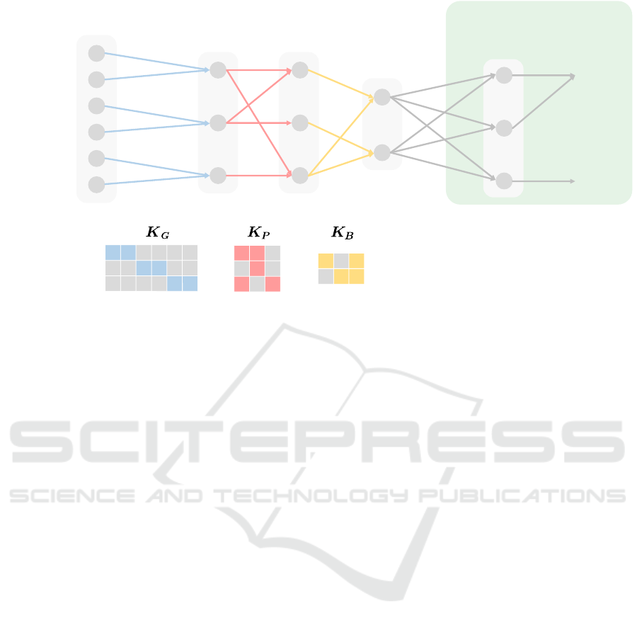
Genes
Input
layer
Knowledge
matrices
transition transition transition
Pathways Biological
processes
Prototype
layer
Output
class 1
class 2
Figure 2: The same example as in Fig. 1 but now realized as a shallow BiGMLVQ. The knowledge matrices K
G
, K
P
, and K
B
represent the biological knowledge of the layer connections according to the structure S and, thus, determine the structure of
the adjustable matrices Ω
1
= Ω
G
, Ω
2
= Ω
P
, and Ω
3
= Ω
B
realizing linear maps between the layers in BiGMLVQ. Further,
the standard output layer of BiDNN is replaced by a prototype layer.
layer-wise discriminating correlation matrices for the
classification task whereas Ω = Ω
B
· Ω
P
· Ω
G
is the
resulting mapping matrix for the BiGMLVQ.
4 EXPERIMENTS
In this section, we empirically evaluate the BiGMLVQ
for predicting prostate cancer severity based on
patient mutation data provided in Elmarakeby et al.
(2021). We compare the performance of our
shallow BiGMLVQ model with the deep biologically-
informed network P-Net (pathway-aware multi-
layered hierarchical network) proposed in that work.
Our results serve as proof of concept for BiGMLVQ.
4.1 Data Set Description and
Experimental Setup
The original prostate cancer data set from Elmarakeby
et al. (2021) involves genomic profiles of
1, 013 patients, given by the somatic mutation
(changes in the sequence), copy number amplification
(increase in a genome fragment) and copy number
deletion (missing DNA segment) of 9, 229 genes in
total. The aim is to distinguish Castration Resistant
Prostate Cancer (CRPC) from primary cancers,
whereby 333 and 680 patient profiles were available
per class, respectively. Prior biological knowledge
is obtained from the Reactome database, grouping
genes into a hierarchy of increasingly coarse pathways
and eventually biological processes. The data set
and pathways information is publicly available, we
simply refer to the links provided by the authors
and explicitly mention the files we used (see data
availability statement).
After preprocessing, we remain with
1, 011 patients (two non-CRPC patients were
removed due to missing mutation information),
1, 573 genes (considering only those for which
complete data, i. e., mutation, copy number variation,
and pathway assignment information are available)
and 186 pathways. To keep the approach as simple
as possible, in this first demonstration, we do not
decompose the pathways into their functionalities as it
was done in the original publication.
This corresponds to BiGMLVQ with two hidden
layers: a gene layer L
1
= L
G
and a pathway layer L
2
=
L
P
(cf. Fig. 2 omitting the biological process layer).
The input layer has a dimensionality of 3 × 1, 573
according to the mutation, deletion, and amplification
information available for each gene. For the pathway
layer, 186 pathways are considered in agreement with
Elmarakeby et al. (2021). Thus we get
Ω = Ω
P
· Ω
G
(9)
as the resulting mapping matrix for the BiGMLVQ
with the decomposition matrices Ω
G
∈ R
3·1573×1573
and Ω
P
∈ R
1573×186
. The corresponding structure
matrices K
G
and K
P
are determined according to
Elmarakeby et al. (2021).
The mutation entries in the input data take binary
values indicating the occurrence of a mutation for the
BIOINFORMATICS 2024 - 15th International Conference on Bioinformatics Models, Methods and Algorithms
362

considered gene whereas copy number variation and
deletions just count these events. For the classification
layer, i. e., the prototype layer, we have chosen one
or three prototypes per class such that a linear and a
non-linear classifier is realized, respectively.
The BiGMLVQ-model is implemented in
ProtoTorch (Ravichandran, 2020). The test split
from Elmarakeby et al. (2021) was adopted while the
training and validation splits were generated randomly
with the same ratio as they were using for the P-Net
model. BiGMLVQ was trained by SGDL using the
Adam optimizer. This procedure was repeated 20
times to achieve statistically valid results and to obtain
robustness information of the model.
4.2 Results and Discussion
The results of our BiGMLVQ together with the
performance of P-Net are listed in Table 1. We
recognize in this table that BiGMLVQ significantly
outperforms the deep network P-Net, even though it
is less complex and only a linear feature processing
takes place by the mapping matrices Ω
k
. Thereby, it
is interesting to note that the test performance with
one prototype is slightly better than that of the larger
model with three prototypes. However, this difference
is not statistically significant. If we take a closer look
at the corresponding training accuraccies of 95.3% and
94.7% respectively, we can attribute this behavior to a
model overfitting for the larger model.
BiGMLVQ also provides direct insight into the
importance of features. Fig. 3 shows the reduced
classification correlation matrix Λ
P
with the 10 genes
that most influence the decision process. The most
important genes are determined by using the CIP
Eq. (6) of Λ
P
. It should be noted that our findings
are similar to those of Elmarakeby et al. (2021). The
genes AR, PTEN and FGFR1, among others, are also
said to be decisive in P-Net. Interestingly, the negative
classification correlation between the genes AR and
FGFR1 indicates that opposing these genes supports a
better class discrimination. Moreover, especially the
mutation and amplification of AR and the mutation
value of PTEN are relevant, which can be read directly
from Λ
1
= Λ
G
, see Fig. 4. Yet on average all three
input types (mutation, amplification, and deletion)
have an influence on the class discrimination, with
the influence of amplification values being the largest
(see Fig. 5).
Remark 5. If we compare the BiGMLVQ with
the standard GMLVQ where the mapping matrix
Ω
GMLVQ
∈ R
186×4719
is learned without restrictions
a clear overfitting of the GMLVQ can be observed:
The respective GMLVQ test accuracy is only 0.860 ±
Table 1: Averaged test results given in precentage together
with standard deviation obtained by BiGMVLQ with one
and three Prototypes per Class (PpC) compared to the P-Net
results taken from Elmarakeby et al. (2021). Averaging was
done by 20 independent runs.
BiGMLVQ P-Net
1 PpC 3 PpC
Accuracy 93.6 ± 1.4 92.1 ± 1.5 83.8
Recall 84.8 ± 2.8 83.5 ± 4.4 76.3
Precision 95.5 ± 3.4 92.3 ± 3.8 75.0
F1-measure 89.8 ± 2.1 87.5 ± 2.5 75.5
0.032 , whereas the corresponding training accuracy is
0.986 ±0.002 for a simple GMLVQ model with only
one prototype per class. Hence, looking at the high test
performance of BiGMLVQ, we can conclude that the
structure information used in BiGMLVQ reduces the
danger of overfitting by restricting the parameters to
learn meaningful connections while achieving high
performance. In our experiment, the used matrix
Ω from Eq. (9) contains only 1.47% non-zero (i.e.
adjustable) entries.
Beside this structural constraint, an evaluation of
the importance of, e. g., the genes, is only meaningful
due the provided knowledge-driven structure. Yet, an
interpretation of the learned mapping remains at least
difficult.
5 CONCLUSIONS
In this work, we propose a biologically-informed
shallow neural network – BiGMLVQ based on
the principle of learning vector quantization. The
model consists of adaptive linear layers whose
topological structure reflects the biological domain
knowledge of genes, pathways, and corresponding
biological processes. The nonlinear classification
ability of BiGMLVQ is ensured by the subsequent
prototype layer, which realizes a provably robust
and interpretable classification scheme as known
from learning vector quantization. Furthermore, the
adaptive linear layers allow an direct interpretation
in terms of correlation analysis supporting class
separation. Otherwise, in the application phase,
the combination of these linear layers simply
yields a summarized linear map allowing efficient
computations.
We have shown in the experiment that this shallow
BiGMLVQ network is capable of achieving better
results than a biologically-informed deep neural
network, which has higher computational complexity
due to the non-linearity of each layer and requires
advanced tools for interpretation.
It is worth noting that for BiGMLVQ, we can
Biologically-Informed Shallow Classification Learning Integrating Pathway Knowledge
363

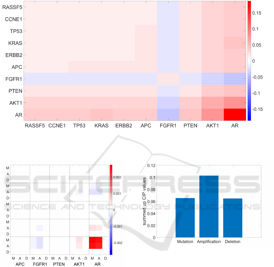
Figure 3: Layer-wise classification correlation matrix Λ
1
= Λ
G
reduced to the 10 most influential genes according to the
layer-wise CIP λ
1
of the first layer L
1
= L
G
. According to this visualization, the genes AR, PTEN, AKT1, and FGFR1 are
depicted to be decisive for class separation, which is in nice agreement with the findings for the P-Net in Elmarakeby et al.
(2021).
Figure 4: Overall classification correlation matrix Λ
regarding the full mapping Ω = Ω
P
· Ω
G
for the input
features, but considering only the five most important genes
according to the (overall) CIP λ for better visibility of the
effects. We observe that for different genes the importance
of mutation, amplification, and deletion values varies.
apply all the variants developed for standard GMLVQ
including border-sensitive learning, transfer learning
(Kästner et al., 2012) or one-class-classification
learning (Staps et al., 2022), which is planned for
future research. Additionally, in future work, we
will investigate the (layer-wise) classification mapping
correlation matrices ϒ and ϒ
k
as introduced in
Remark 2 and Remark 4 for advanced BiGMLVQ
model evaluation and interpretation.
Figure 5: Summed up classification importance values of Λ
G
for mutation, amplification, and deletion. This visualization
suggests a slightly favored amplification importance for the
class separation in an overall evaluation.
6 DATA AVAILABILITY
The prostate cancer data set was made publicly
available by Elmarakeby et al. (2021) under https:
/ /drive.google.com/uc?id =17nssbdUylkyQY1
ebtxsIw5UzTAd0zxWb.
Particularly, we concentrate on the
information provided in the folder
_database/prostate/processed with the files:
/P1000_final_analysis_set_cross_important_
only for the mutation, P1000_data_CNA_paper
for the deletion and amplification values (copy
BIOINFORMATICS 2024 - 15th International Conference on Bioinformatics Models, Methods and Algorithms
364

number variation (CNV), response_paper
for the labels and the given pathways in
c2.cp.kegg.v6.1.symbols.gmt.
ACKNOWLEDGEMENTS
The authors would like to acknowledge the help and
fruitful discussions of/with Alexander Engelsberger,
Ronny Schubert, and Daniel Staps of the SICIM
at UAS Mittweida (Germany). Further, we thank
Prof. Stefan Simm and Jan Oldenburg, both from
the Institute of Bioinformatics, University Medicine
Greifswald (Germany), for drawing our attention to the
promising topic of biology-informed neural networks
and providing first insights about this research area to
our team.
This work has partially been supported by
the European Social Fund (ESF) and the project
AIMS/IAI-XPRESS of the German aerospace center
(DLR) funded by the German Federal Ministry for
Economic Affairs and Climate Action (BMWK),
funding indicator 50WK2270.
REFERENCES
Bach, S., Binder, A., Montavon, G., Klauschen, F.,
Müller, K.-R., and Samek, W. (2015). On pixel-
wise explanations for non-linear classifier decisions
by layerwise relevance propagation. PLOS One,
10(7):e0130140.
Barredo Arrieta, A., Díaz-Rodríguez, N., Del Ser, J.,
Bennetot, A., Tabik, S., Barbado, A., Garcia, S.,
Gil-Lopez, S., Molina, D., Benjamins, R., Chatila,
R., and Herrera, F. (2020). Explainable artificial
intelligence (xai): Concepts, taxonomies, opportunities
and challenges toward responsible ai. Information
Fusion, 58:82–115.
Biehl, M. (2022). The Shallow and the Deep – A
biased introduction to neural networks and old school
machine learning. University Groningen.
Biehl, M., Hammer, B., and Villmann, T. (2016).
Prototype-based models in machine learning. Wiley
Interdisciplinary Reviews: Cognitive Science, 7(2):92–
111.
Bunte, K., Schneider, P., Hammer, B., Schleif, F.-M.,
Villmann, T., and Biehl, M. (2012). Limited rank
matrix learning, discriminative dimension reduction
and visualization. Neural Networks, 26(1):159–173.
Crammer, K., Gilad-Bachrach, R., Navot, A., and N.Tishby
(2003). Margin analysis of the LVQ algorithm. In
Becker, S., Thrun, S., and Obermayer, K., editors,
Advances in Neural Information Processing (Proc.
NIPS 2002), volume 15, pages 462–469, Cambridge,
MA. MIT Press.
Dash, T., Chitlangia, S., Ahuja, A., and Srinivasan, A. (2022).
A review of some techniques for inclusion of domain-
knowledge into deep neural networks. Nature Scientifi
Reports, 12(1040):1–15.
Elmarakeby, H., Hwang, J., Arafeh, R., Crowdis, J., Gang, S.,
Liu, D., AlDubayan, S., Salari, K., Kregel, S., Richter,
C., Arnoff, T., Park, J., Hahn, W., and Van Allen, E.
(2021). Biologically informed deep neural network for
prostate cancer discovery. Nature, 598:348–352.
Esser-Skala, W. and Fortelny, N. (2023). Reliable
interpretability of biology-inspired deep neural
networks. NPJ Systems Biology and Applications,
9(50):1–8.
Fabregat, A., Jupe, S., Matthews, L., Sidiropoulos, K.,
Gillespie, M., Garapati, P., Haw, R., Jassal, B.,
Korninger, F., May, B., Milacic, M., Roca, C. D.,
Rothfels, K., Sevilla, C., Shamovsky, V., Shorser, S.,
Varusai, T., Viteri, G., Weiser, J., Wu, G., Stein, L.,
Hermjakob, H., and D’Eustachio, P. (2018). The
Reactome Pathway Knowledgebase. Nucleic Acids
Research, 46(D1):D649–D655.
Futia, G. and Vetrò, A. (2020). On the integration of
knowledge graphs into deep learning models for a
more comprehensible AI – Three challenges for future
research. Information, 11(122):1–10.
Gene Ontology Consortium (2004). The Gene Ontology
(GO) database and informatics resource. Nucleic Acids
Research, 32(90001):258D–261.
Goodfellow, I., Bengio, Y., and Courville, A. (2016). Deep
Learning. MIT Press, Cambridge, MA.
Greene, C. S. and Costello, J. C. (2020). Biologically
Informed Neural Networks Predict Drug Responses.
Cancer Cell, 38(5):613–615.
Hartman, E., Scott, A., Karlsson, C., Mohanty, T., Vaara, S.,
Linder, A., Malmström, L., and Malmström, J. (2023).
Interpreting biologically informed neural networks for
enhanced proteomic biomarker discovery and pathway
analysis. Nature Communications, 14(5359):1–13.
Haykin, S. (1994). Neural Networks - A Comprehensive
Foundation. IEEE Press, New York.
Janzing, D., Minorics, L., and Bloebaum, P. (2020).
Feature relevance quantification in explainable AI: A
causal problem. In Proceedings of the Twenty Third
International Conference on Artificial Intelligence and
Statistics (AISTAT), volume 108 of Proceedings of
Machine Learning Research, pages 2907–2916.
Kaden, M., Bohnsack, K., Weber, M., Kudla, M., Gutowska,
K., Blazewicz, J., and Villmann, T. (2021). Learning
vector quantization as an interpretable classifier for
the detection of SARS-CoV-2 types based on their
RNA-sequences. Neural Computing and Applications,
34(1):67–78.
Kanehisa, M. (2000). KEGG: Kyoto Encyclopedia of Genes
and Genomes. Nucleic Acids Research, 28(1):27–30.
Kanehisa, M., Furumichi, M., Sato, Y., Kawashima, M., and
Ishiguro-Watanabe, M. (2023). KEGG for taxonomy-
based analysis of pathways and genomes. Nucleic
Acids Research, 51:D587–D592.
Karniadakis, G., Kevrekidis, I., Lu, L., Perdikaris, P., Wang,
Biologically-Informed Shallow Classification Learning Integrating Pathway Knowledge
365

S., and Yang, L. (2021). Physics-informed machine
learning. Nature Reviews Physics, 2:422–440.
Kästner, M., Riedel, M., Strickert, M., and Villmann,
T. (2012). Class border sensitive generalized
learning vector quantization - an alternative to
support vector machines. Machine Learning
Reports, 6(MLR-04-2012):40–56. ISSN:1865-
3960, http://www.techfak.uni-bielefeld.de/ ˜
fschleif/mlr/mlr_04_2012.pdf.
Kohonen, T. (1988). Learning Vector Quantization. Neural
Networks, 1(Supplement 1):303.
Lisboa, P., Saralajew, S., Vellido, A., Fernández-Domenech,
R., and Villmann, T. (2023). The coming of age of
interpretable and explainable machine learning models.
Neurocomputing, 535:25–39.
Lundberg, S. and Lee, S.-I. (2017). A unified approach
to interpreting model predictions. In Guyon, I.,
Luxburg, U. V., Bengio, S., Wallach, H., Fergus, R.,
Vishwanathan, S., and Garnett, R., editors, Advances
in Neural Information Processing Systems, volume 30,
pages 4768–4777. Curran Associates, Inc.
Mohannazadeh Bakhtiari, M. and Villmann, T. (2023).
The geometry of decision borders between affine
space prototypes for nearest prototype classifiers.
In Rutkowski, L., Scherer, R., Pedrycz, M.
K. W., Tadeusiewicz, R., and Zurada, J., editors,
Proceedings of the International Conference on
Artificial Intelligence and Soft Computing (ICAISC),
volume 14125 of LNAI, pages 134–144.
Montavon, G., Binder, A., Lapuschkin, S., Samek, W.,
and Müller, K.-R. (2019). Layer-Wise Relevance
Propagation: An Overview, pages 193–209. Springer
International Publishing, Cham.
Murdoch, W., Singh, C., Kumbiera, K., Abbasi-Aslb,
R., and Yu, B. (2019). Interpretable machine
learning: definitions, methods, and applications.
Proccedings of the National Academy od Science
(PNAS), 116(44):22071–22080.
Ravichandran, J. (2020). Prototorch. https://github.com/si-c
im/prototorch.
Ravichandran, J., Kaden, M., and Villmann, T. (2022).
Variants of recurrent learning vector quantization.
Neurocomputing, 502(8–9):27–36.
Rudin, C., Chen, C., Chen, Z., Huang, H., Semenova, L.,
and Zhong, C. (2022). Interpretable machine learning:
Fundamental principles and 10 grand challenges.
Statistics Survey, 16:1–85.
Samek, W., Monatvon, G., Vedaldi, A., Hansen, L.,
and Müller, K.-R., editors (2019). Explainable
AI: Interpreting, Explaining and Visualizing Deep
Learning, number 11700 in LNAI. Springer.
Samek, W., Montavon, G., Lapuschkin, S., Anders, C., and
Müller, K.-R. (2021). Explaining deep neural networks
and beyond: A review of methods and applications.
Proceedings of the IEEE, 109(3):247–278.
Saralajew, S., Holdijk, L., Rees, M., and Villmann, T.
(2019). Robustness of generalized learning vector
quantization models against adversarial attacks. In
Vellido, A., Gibert, K., Angulo, C., and Guerrero, J.,
editors, Advances in Self-Organizing Maps, Learning
Vector Quantization, Clustering and Data Visualization
– Proceedings of the 13th International Workshop
on Self-Organizing Maps and Learning Vector
Quantization, Clustering and Data Visualization,
WSOM+2019, Barcelona, volume 976 of Advances
in Intelligent Systems and Computing, pages 189–199.
Springer Berlin-Heidelberg.
Sato, A. and Yamada, K. (1996). Generalized learning
vector quantization. In Touretzky, D. S., Mozer, M. C.,
and Hasselmo, M. E., editors, Advances in Neural
Information Processing Systems 8. Proceedings of the
1995 Conference, pages 423–9. MIT Press, Cambridge,
MA, USA.
Schneider, P., Bunte, K., Stiekema, H., Hammer, B.,
Villmann, T., and Biehl, M. (2010). Regularization
in matrix relevance learning. IEEE Transactions on
Neural Networks, 21(5):831–840.
Schneider, P., Hammer, B., and Biehl, M. (2009). Adaptive
relevance matrices in learning vector quantization.
Neural Computation, 21:3532–3561.
Semenova, L., Rudin, C., and Parr, R. (2022). On
the existence of simpler machine learning models.
In ACM Conference on Fairness, Accountability,
and Transparency (FAccT’22), pages 1827–1858.
Association for Computing Machinery.
Shrikumar, A., Greenside, P., and Kundaje, A. (2017).
Learning important features through propagating
activation differences. In Proceedings of the
34th International Conference on Machine Learning
(ICML), volume 70, pages 3145–3153.
Snel, B. (2000). STRING: A web-server to retrieve and
display the repeatedly occurring neighbourhood of a
gene. Nucleic Acids Research, 28(18):3442–3444.
Staps, D., Schubert, R., Kaden, M., Lampe, A., Hermann,
W., and Villmann, T. (2022). Prototype-based one-
class-classification learning using local representations.
In Proceedings of the IEEE International Joint
Conference on Neural Networks (IJCNN) - Padua, Los
Alamitos. IEEE Press.
Torun, F., Winter, S., Riese, S. D. F., Vorobyev, A.,
Mueller-Reif, J., Geyer, P., and Strauss, M. (2022).
Transparent exploration of machine learning for
biomarker discovery from proteomics and omics data.
Journal of Proteome Research, 22(2):359–367.
Villmann, T., Biehl, M., Villmann, A., and Saralajew,
S. (2017a). Fusion of deep learning architectures,
multilayer feedforward networks and learning
vector quantizers for deep classification learning.
In Proceedings of the 12th Workshop on Self-
Organizing Maps and Learning Vector Quantization
(WSOM2017+), pages 248–255. IEEE Press.
Villmann, T., Bohnsack, A., and Kaden, M. (2017b). Can
learning vector quantization be an alternative to SVM
and deep learning? Journal of Artificial Intelligence
and Soft Computing Research, 7(1):65–81.
von Rueden, L., Mayer, S., Georgiev, K. B. B., Giesselbach,
S., Heese, R., Kirsch, B., Pick, J. P. A., Walczak, R.
R. M., Garcke, J., Bauckhage, C., and Schuecker, J.
(2023). Informed machine learning – A taxonomy and
survey of integrating prior knowledge into learning
BIOINFORMATICS 2024 - 15th International Conference on Bioinformatics Models, Methods and Algorithms
366

systems. IEEE Transactions on Knowledge and Data
Enginiering, 35(1):614–633.
Wysocka, M., Wysocki, O., Zufferey, M., Landers, D.,
and Freitas, A. (2023). A systematic review of
biologically-informed deep learning models for cancer:
fundamental trends for encoding and interpreting
oncology data. BMC Bioinformatics, 24(198):1–31.
Zhou, T., Lopez Droguett, E., and Mosleh, A. (2022).
Physics-informed deep learning: A promising
technique for system reliability assessment. Applied
Soft Computing, 126(109217):1–21.
Biologically-Informed Shallow Classification Learning Integrating Pathway Knowledge
367