Visualization of the Basis for Decisions by Selecting Layers Based on

Model's Predictions Using the Difference Between Two Networks

Takahiro Sannomiya

and Kazuhiro Hotta

Meijo University, Nagoya, Japan

Keywords: Explainable AI, Neural Network Interpretability, Class Activation Map.

Abstract: Grad-CAM and Score-CAM are methods to improve the interpretation of CNNs whose internal behaviour is

opaque. These methods do not select which layer to use, but simply use the final layer to visualize the basis

of the decision. However, we wondered whether this was really appropriate, and wondered whether there

might be important information hidden in layers other than the final layer in making predictions. In the

proposed method, layers are selected based on the prediction probability of the model, and the basis of

judgment is visualized. In addition, by taking the difference between the model that has been trained slightly

to increase the confidence level of the model's output class and the model before training, the proposed method

performs a process to emphasize the parts that contributed to the prediction and provides a better quality basis

for judgment. Experimental results confirm that the proposed method outperforms existing methods in two

evaluation metrics.

1 INTRODUCTION

In recent years, deep learning has made dramatic

progress and is being actively studied around the

world. AlexNet based on Convolutional Neural

Networks (CNNs) was a pioneer in this field. Since

AlexNet was introduced, research has been conducted

on image classification, object detection, and image

generation using CNNs. However, CNNs are opaque

in their internal operation, making it difficult to

interpret the basis for the model's decisions.

Understanding the basis for model’s decisions is

essential for achieving better accuracy and for making

important decisions such as pathological diagnosis

and object detection.

Various methods have been proposed to solve this

problem. For example, CAM weights the feature map

obtained by Global Average Pooling (GAP) to make

it easier to see the points that the CNN is focusing on.

However, this method is not applicable to models that

do not use GAP. Therefore, Grad-CAM was proposed

which substitutes the weights with the gradient.

Score-CAM was also proposed in which the weights

are obtained from the prediction probabilities. Both

methods eliminate model constraints, but they use

https://orcid.org/0009-0005-3644-381X

https://orcid.org/0000-0002-5675-8713

only the final layer to visualize the basis for decisions,

and do not take into account the presence of important

information in other layers that may be relevant to

predictions.

In this paper, the layers are selected based on the

model's prediction probability, and the basis of

judgment is visualized. In addition, by taking the

difference between the model before training and the

model that has been trained slightly to increase the

confidence level of the model's output class, we

perform a process to emphasize the parts that

contributed to the prediction and provide a better

quality basis for judgment.

In our experiments, we evaluated and discussed

the results on 3,000 images randomly selected from

the validation dataset in ImageNet, which consists of

1,000 classes of animals and vehicles, etc. We

evaluated the results using Insertion and Deletion,

and our method achieved better accuracy than the

conventional methods on both measures. The

accuracy of our method is higher than that of

conventional methods.

The paper is organized as follows. Section 2

describes related works. Section 3 describes the

details of the proposed method. Section 4 shows

370

Sannomiya, T. and Hotta, K.

Visualization of the Basis for Decisions by Selecting Layers Based on Model’s Predictions Using the Difference Between Two Networks.

DOI: 10.5220/0012419300003654

Paper published under CC license (CC BY-NC-ND 4.0)

In Proceedings of the 13th International Conference on Pattern Recognition Applications and Methods (ICPRAM 2024), pages 370-377

ISBN: 978-989-758-684-2; ISSN: 2184-4313

experimental results. Section 5 describes the ablation

study. Section 6 is for conclusions and future works.

2 RELATED WORKS

In this section, we discuss related works. Section 2.1

describes Grad-CAM, and Section 2.2 describes

Score-CAM.

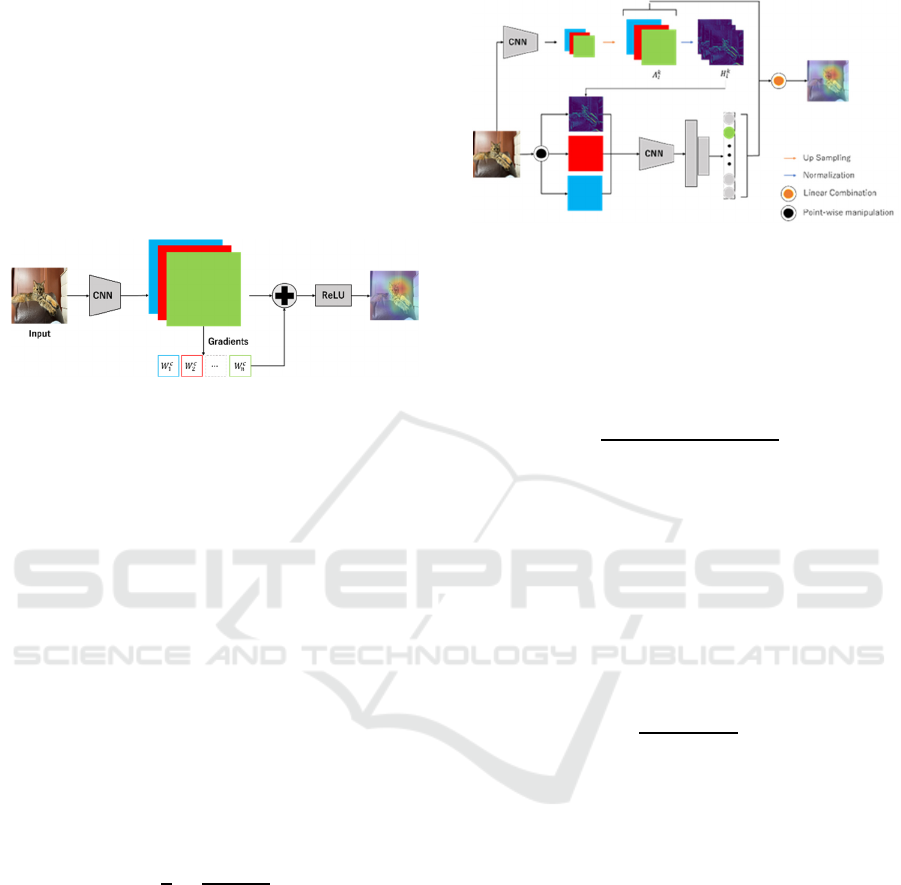
2.1 Grad-CAM

Figure 1: Overview of Grad-CAM.

Grad-CAM is a method in which the weighting

method for feature maps is replaced by gradients so

that the basis of judgment can be visualized even in

models that do not include Global Average Pooling.

An overview of Grad-CAM is shown in Figure 1.

Grad-CAM uses the gradient calculated from the

feature maps at the last layer to visualize the basis for

decisions. The blue-red-green maps in Figure 1

represent different feature maps, and the gradient is

calculated from each feature map. Grad-CAM is

computed as follows.

𝐿



𝑅𝑒𝐿𝑈𝛼





𝐴





(1)

where 𝐴

,



represents the feature map 𝐴



in the kth

channel and position 𝑖,𝑗. 𝛼





is calculated from the

gradient as follows.

𝛼







𝑍



𝜕𝑆



𝜕

𝑓



𝑥,𝑦

,

(2)

where Z is the normalization constant and 𝑆



represents the prediction probability of class 𝑐. 𝛼





represents how much 𝑆



changed when the pixel at

coordinate 𝑖,𝑗 in feature map 𝑘 changed. Thus, the

coordinates 𝑖,𝑗 with large 𝛼





have positive effect

on the prediction. In addition, the 𝑅𝑒𝐿𝑈 function in

equation (1) is used to cut off the negative component,

making the basis for the decision easier to understand.

However, Grad-CAM only uses information from the

final layer, so it cannot take into account the presence

of important information in other layers.

2.2 Score-CAM

Figure 2: Overview of Score-CAM.

Score-CAM is a method that replaces the weighting

of feature maps with predictive probabilities. If an

image 𝑋 is fed into the CNN and the feature map of

the 𝑘 th channel in layer 𝑙 is 𝐴





, the normalized

feature map 𝐻





is calculated as follows.

𝐻







𝐴





𝑚𝑖𝑛

𝐴







𝑚𝑎𝑥

𝐴





min 

𝐴







(3)

Next, the input image multiplied by 𝐻





is fed into

the CNN, and 𝑆



is calculated from the difference

with the original image. If the predicted probability of

class 𝑐 is 𝑓



when the image is fed into the CNN,𝑆



is computed as follows.

𝑆





𝑓



𝑋 ∘ 𝐻







𝑓



𝑥 (4)

We normalize the obtained 𝑆



so that the sum is 1,

and 𝛼





is computed as follows.

𝛼







exp



𝑆







∑

exp 𝑆









(5)

By multiplying the 𝛼





to the feature map, a heat map

is obtained as shown in the following equation.

𝐿





𝑅𝑒𝐿𝑈𝛼





𝐴







(6)

Score-CAM has the same problem as Grad-CAM

because it only uses information from the final layer.

Therefore, the proposed method takes the difference

between the two networks and emphasizes the

locations that had a positive impact on the prediction

probability. It then selects a layer based on the

model's prediction probability and visualizes the basis

for the decision.

Visualization of the Basis for Decisions by Selecting Layers Based on Model’s Predictions Using the Difference Between Two Networks

371

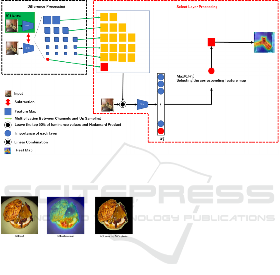
Figure 3: Overview of the proposed method.

3 PROPOSED METHOD

Figure 4: Example of top 50% of the importance W.

Figure 3 shows an overview of the proposed method.

The proposed method consists of “difference

processing” and “select layer processing”. In

difference processing, at first, an image is fed into

network, which has already been trained on the

ImageNet, and it is trained 𝑁 times so that the

probability for the predicted class increases (The area

shown as green in the upper left of Figure 3). After

that, we take the difference 𝑑





(the blue map in Figure

3) between network trained 𝑁 times and the original

network for each channel at all layers. Next, the

differenced feature map is resized to 224  224

pixels so that the image size is the same as the input

image. Although it would be desirable to consider the

relationship between channels at each layer, the

computational complexity would be enormous, so

here we summed the channels at all layers.

By this process, the yellow and red maps in Figure

3 are obtained. However, for clarity, the feature map

obtained from the final output is colored red here.

In Select Layer Processing, only the pixels in the

top 50% of the feature map values of the feature map

are kept in each layer as shown in Figure 3. They are

multiplied with the original image. This is then input

to the original network and the importance of each

feature map is calculated. If the predicted probability

of class 𝑐 is 𝑌



when the original image is input, and

the predicted probability of class 𝑐 is 𝑌





when an

image in which only the top 50% of the feature map

in layer 𝑙 is retained and multiplied with the original

image is input, the importance 𝑊





is as follows.

where 1 is added to 𝑊





to prevent the importance

from being negative.

𝑊





1𝑌





𝑌





(7)

Example of this process is shown in Figure 4.

Figure 4 (a) is an input image and (b) is the image

obtained by summing the feature maps at a certain

layer across channels. Figure 4 (c) shows the image

obtained by leaving the top 50% of the feature map

values and multiplying them with the input image.

The importance 𝑊





is obtained by creating the image

with all outputs, and it is fed into network.

Finally, only the feature map with the highest

importance 𝑊





calculated from the prediction

probability is used as the basis for the final decision.

ICPRAM 2024 - 13th International Conference on Pattern Recognition Applications and Methods

372

This method allows us to take into account

information outside of the final layer while

emphasizing the areas that contributed to the

predicted probability.

4 EXPERIMENTS

4.1 Experimental Settings

In the following experiments, we used 3,000

randomly selected images from the validation set in

the ImageNet dataset. However, those images are the

same for all methods. The images were resized to

224  224 pixels and fed into the network. In this

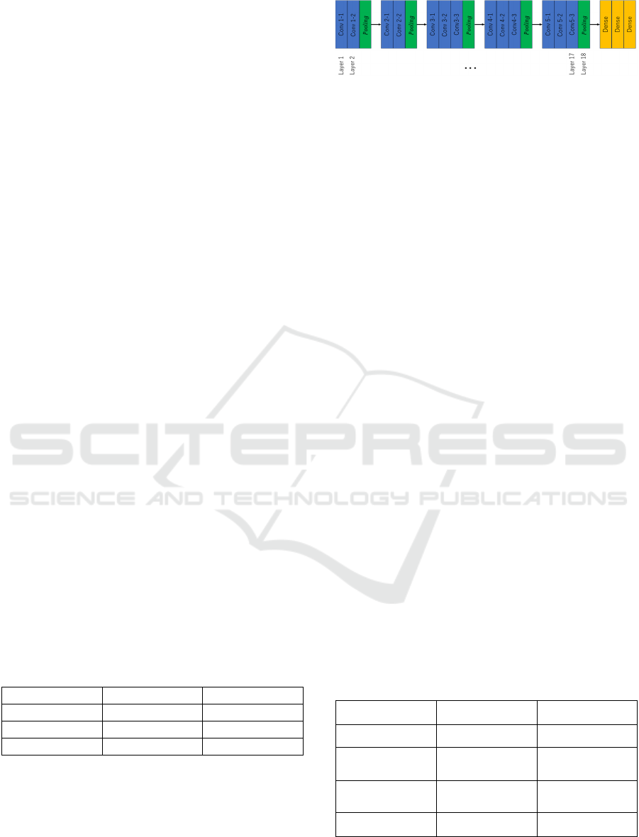
paper, we use VGG16 as the network. In this paper,

VGG16 is used in the experiments because related

works also used it. The structure of VGG16 and

definition of “Layer” is shown in Fig.7. We define

that the first layer is layer 1 and the final layer is layer

18, and one of those layers is used for visualization.

Next, we describe the evaluation metrics. We use

Insertion and Deletion. Insertion is an evaluation

metric that measures the increase in the model's

prediction probability when pixels are inserted in the

order of the magnitude in the visualization image.

This metric measures the increase in the model's

predictive probability as more pixels are inserted,

with a higher AUC (area under the probability curve)

indicating a more adequate explanation.

Deletion is a metric that measures the degree to

which the model's predictive probability decreases as

pixels are removed from the visualization image in

order of increasing high value of visualization image.

This metric measures the decrease in the model's

predictive probability as more pixels are removed.

Lower AUC curve indicates a better explanation.

4.2 Experimental Results

Table1: Comparison results.

Metho

Insertion [%] Deletion [%]

Grad-CAM 36.00 5.43

Score-CAM 36.69 5.21

Ours 40.21 4.79

Comparison results between Grad-CAM, Score-

CAM, and the proposed method are shown in Table

1. The best results are shown in red. We see that the

proposed method improves the accuracy of Insertion

by 4.21% and 3.52% compared to Grad-CAM and

Score-CAM. In Deletion, the proposed method

improves accuracy by 0.64% and 0.42%,

Figure 5: Definition of "Layer" of VGG16 in this paper.

respectively. We will discuss the factors behind the

improvement in accuracy using the visualization

results. Figure 6 and 7 shows an example of

visualization results and the Insertion Curve and

Deletion Curve for the visualization results to confirm

whether the basis for judgment can be visualized.

Here, "Layer" under "Ours" indicates the number of

the layer used. The definition of “Layer” is already

shown in Figure 5. As shown in Figure 6 and 7, we

see that from (a) to (e) provide better quality

visualization than the other methods. In particular, (a)

and (e) show an earlier increase in prediction

probability for the Insertion Curve and an earlier

decrease in prediction probability for the Deletion

Curve compared to the other methods. The

visualization results show that the model is more

successful than the other method. This can be

attributed to the fact that the layer selection was

performed based on the prediction probability, after

taking the difference between the two networks and

highlighting the areas that had a positive impact on

the prediction probability. The relationship between

difference processing and accuracy is discussed in the

Section 5.

5 ABLATION STUDY

In this section, we investigate the utilization rate of

each layer and the validity of the difference of two

networks as an Ablation Study.

5.1 Effectiveness of Difference

Table 2: Comparison of accuracy w/o the difference.

Metho

Insertion [%] Deletion [%]

Score-CAM 36.69 5.21

Score-CAM

w/ difference

39.04 5.00

Ours w/o

difference

36.51 4.83

Ours 40.21 4.79

This section investigates whether the difference of

two networks contributes to improve the accuracy.

Visualization of the Basis for Decisions by Selecting Layers Based on Model’s Predictions Using the Difference Between Two Networks

373

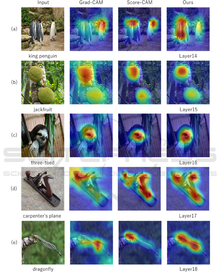
Figure 6: Visualization results by each method.

The results are shown in Table 2. Table 2 shows the

results of the proposed method with and without the

difference of two networks. When the difference

processing is eliminated from the proposed method,

the accuracy of Insertion and Deletion decreases by

3.7% and 0.04%. This shows the effectiveness of the

difference of two networks.

ICPRAM 2024 - 13th International Conference on Pattern Recognition Applications and Methods

374

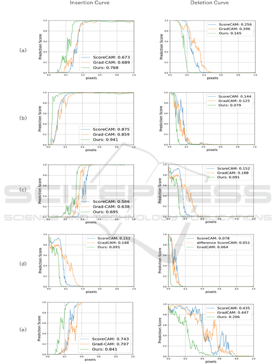
Figure 7: Insertion curve and Deletion curve by each method.

Visualization of the Basis for Decisions by Selecting Layers Based on Model’s Predictions Using the Difference Between Two Networks

375

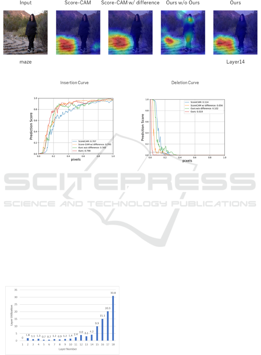
Figure 8: Comparison of accuracy with and without difference.

Figure 9: Comparison of Insertion Curve and Deletion Curve with and without difference.

We also show the accuracy of Score-CAM with

and without the difference. When difference

processing is applied to Score-CAM, the accuracy

improved by 2.35% for Insertion and 0.21% for

Deletion. respectively. This is because the difference

between two networks can emphasize the points that

contribute to classification.

Figure 8 and 9 also shows that difference

processing improved the quality of the visualization

by preventing the heatmap from going to locations

other than the objects predicted by the model.

Therefore, we see that difference of two networks

contributes to improve the accuracy.

5.2 Utilization Rates of Each Layer

Figure 10: Utilization rates of each layer.

In this section, we investigate the utilization of each

layer. The same 3,000 images from the ImageNet

validation set as section 4 are used to show the

utilization of each layer. Figure 10 shows that layers

other than the final layer are also used. Note that the

definition of “Layer” is shown in Figure 5. Figure 10

indicates that the important information for prediction

is not always in the final layer. Conventional methods

such as Grad-CAM and Score-CAM used the

information from only the final layer, but the

proposed method selects layers based on prediction

probability rather than only the final layer, and this

derived better visualization results.

6 CONCLUSIONS

Conventional methods for visualization of the basis

for decision making use only the final layer for

visualization, and they do not take into account

important information hidden in other layers that are

relevant to classification. In this paper, we propose a

method to take into account important information

hidden in layers other than the final layer by selecting

layers based on the prediction probability of the

model, while highlighting the parts that contributed to

the prediction by taking the difference between the

ICPRAM 2024 - 13th International Conference on Pattern Recognition Applications and Methods

376

original model and the model that was trained slightly

to increase the confidence level of the output class.

As a result, we achieved the accuracy improvement in

two evaluation measures. The visualization results

also confirmed that the visualization of the basis for

decision-making was of better quality than that of

existing methods.

ACKNOWLEDGEMENTS

This research is partially supported by JSPS

KAKENHI Grant Number 22H04735.

REFERENCES

Krizhevsky, A., Sutskever, I., & Hinton, G. E. (2012).

Imagenet classification with deep convolutional neural

networks. Advances in Neural Information Processing

Systems, pp. 1097-1105.

LeCun, Y., Boser, B., Denker, J. S., Henderson, D.,

Howard, R. E., Hubbard, W., & Jackel, L. D. (1989).

Backpropagation Applied to Handwritten Zip Code

Recognition. Neural Computation, 1(4), pp. 541-551.

Wang, F., Jiang, M., Qian, C., Yang, S., Li, C., Zhang, H.,

... & Tang, X. (2017). Residual Attention Network for

Image Classification. In Proceedings of The IEEE

Conference on Computer Vision and Pattern

Recognition, pp. 3156-3164.

Szegedy, C., Liu, W., Jia, Y., Sermanet, P., Reed, S.,

Anguelov, D., ... & Rabinovich, A. (2015). Going

Deeper with Convolutions. In Proceedings of The IEEE

Conference on Computer Vision and Pattern

Recognition, pp. 1-9.

Liu, W., Anguelov, D., Erhan, D., Szegedy, C., & Reed, S.,

(2016) SSD: Single Shot Multibox Detector.

In Proceedings of European Conference on Computer

Vision, pp. 21-37.

Redmon, J., Divvala, S., Girshick, R., & Farhadi, A. (2016).

You only look once: Unified, Real-Time Object

Detection. In Proceedings of The IEEE Conference on

Computer Vision and Pattern Recognition, pp. 779-788.

Redmon, J., & Farhadi, A. (2017). YOLO9000: Better,

Faster, Stronger. In Proceedings of The IEEE

Conference on Computer Vision and Pattern

Recognition, pp. 7263-7271.

Girshick, R., Donahue, J., Darrell, T., & Malik, J. (2014).

Rich feature hierarchies for accurate object detection

and semantic segmentation. In Proceedings of The

IEEE Conference on Computer Vision and Pattern

Recognition, pp. 580-587.

Girshick, R. (2015). Fast R-CNN. In Proceedings of The

IEEE International Conference on Computer Vision, pp.

1440-1448.

Goodfellow, I., Pouget-Abadie, J., Mirza, M., Xu, B.,

Warde-Farley, D., Ozair, S., ... & Bengio, Y. (2014).

Generative Adversarial Nets. Advances in Neural

sInformation Processing Systems, pp. 2672-2680.

Radford, A., Metz, L., & Chintala, S. (2015). Unsupervised

Representation Learning with Deep Convolutional

Generative Adversarial Networks. In Proceedings of

The International Conference on Learning

Representations.

Isola, P., Zhu, J. Y., Zhou, T., & Efros, A. A. (2017). Image-

to-Image Translation with Conditional Adversarial

Networks. In Proceedings of The IEEE Conference on

Computer Vision and Pattern Recognition, pp. 1125-

1134.

Zhou, B., Khosla, A., Lapedriza, A., Oliva, A., & Torralba,

A. (2016). Learning Deep Features for Discriminative

Localization. In Proceedings of The IEEE Conference

on Computer Vision and Pattern Recognition, pp.

2921-2929.

Selvaraju, R. R., Cogswell, M., Das, A., Vedantam, R.,

Parikh, D., & Batra, D. (2017). Grad-cam: Visual

Explanations from Deep Networks via Gradient-based

Localization. In Proceedings of The IEEE International

Conference on Computer Vision, pp. 618-626.

Wang, H., Wang, Z., Du, M., Yang, F., Zhang, Z., Ding,

S., ... & Hu, X. (2020). Score-CAM: Score-Weighted

Visual Explanations for Convolutional Neural

Networks. In Proceedings of The IEEE/CVF

Conference on Computer Vision and Pattern

Recognition Workshops, pp. 24-25.

Russakovsky, O., Deng, J., Su, H., Krause, J., Satheesh, S.,

Ma, S., ... & Fei-Fei, L. (2015). Imagenet Large Scale

Visual Recognition Challenge. International Journal of

Computer Vision, Vol.115, pp. 211-252.

Visualization of the Basis for Decisions by Selecting Layers Based on Model’s Predictions Using the Difference Between Two Networks

377