Enhancing Manufacturing Quality Prediction Models Through the

Integration of Explainability Methods

Dennis Gross

, Helge Spieker

, Arnaud Gotlieb

and Ricardo Knoblauch

Simula Research Laboratory, Oslo, Norway

Ecole Nationale Sup

erieure d’Arts et M

etiers, Aix-en-Provence, France

Keywords:

Industrial Applications of Machine Learning, Explainable Machine Learning.

Abstract:

This research presents a method that utilizes explainability techniques to amplify the performance of machine

learning (ML) models in forecasting the quality of milling processes, as demonstrated in this paper through a

manufacturing use case. The methodology entails the initial training of ML models, followed by a ﬁne-tuning

phase where irrelevant features identiﬁed through explainability methods are eliminated. This procedural re-

ﬁnement results in performance enhancements, paving the way for potential reductions in manufacturing costs

and a better understanding of the trained ML models. This study highlights the usefulness of explainability

techniques in both explaining and optimizing predictive models in the manufacturing realm.

1 INTRODUCTION

Milling is a subtractive manufacturing process that

involves the removal of material from a workpiece

to produce a desired shape and surface ﬁnish. In

this process, a cutting tool known as a milling cutter

rotates at high speed and moves through the work-

piece, removing material. The workpiece is typi-

cally secured on a table that can move along mul-

tiple axes, allowing for various orientations and an-

gles to be achieved (Fertig et al., 2022). The energy

consumption during the milling process can vary sig-

niﬁcantly based on several factors, including the spe-

ciﬁc setup and the materials being processed. How-

ever, it is often considered to be a relatively energy-

intensive process. Being able to foresee and avert

potential quality issues means that less energy is ex-

pended and fewer resources are wasted on creating

defective parts, which would otherwise be rejected or

require reworking (Pawar et al., 2021).

Machine learning (ML) models are capable of

identifying patterns and structures in data to make

predictions without being directly programmed to do

so. These models can be a useful tool in forecast-

ing the ﬁnal quality of a workpiece at the end of

the milling process, helping to improve both the ef-

ﬁciency and the reliability of the manufacturing pro-

cess (Mundada and Narala, 2018).

Lack of Data. However, the available milling ex-

periment data is typically small because the costs for

each manufacturing experiment are very high (Postel

et al., 2020). This lack of data makes it difﬁcult to

learn ML models to predict the workpiece quality.

Explainability Problem. Even if abundant data

were available, utilizing complex ML models, such

as deep neural network models, presents a signiﬁ-

cant challenge due to their “black box” nature. This

term denotes the lack of transparency in understand-

ing these models’ internal workings, which often re-

main inaccessible or unclear (Kwon et al., 2023).

In the realm of turning process quality prediction,

an explainability problem arises when practitioners

and stakeholders can not fully understand the predic-

tions given by these models due to their complex and

opaque nature.

Leveraging Explainability Techniques for Op-

timized Model Training. Explainability methods

are, therefore, crucial in unraveling the complex pre-

diction mechanisms embedded within ML models.

Furthermore, they facilitate enhanced performance of

ML models by identifying and addressing potential

inefﬁciencies, thereby steering optimization efforts

more effectively (Bento et al., 2021; Sun et al., 2022).

898

Gross, D., Spieker, H., Gotlieb, A. and Knoblauch, R.

Enhancing Manufacturing Quality Prediction Models Through the Integration of Explainability Methods.

DOI: 10.5220/0012417800003636

Paper published under CC license (CC BY-NC-ND 4.0)

In Proceedings of the 16th International Conference on Agents and Artiﬁcial Intelligence (ICAART 2024) - Volume 3, pages 898-905

ISBN: 978-989-758-680-4; ISSN: 2184-433X

Approach. We use less computational processing-

intense ML models, such as decision tree regression

or gradient boosting regression, and improve their

performance via explainability methods. We do this

by training these models on a milling dataset, iden-

tifying the important features for these models for

their predictions, removing the less important features

from them, and retraining a new model on stretch

on the feature-pruned data set. Our results show, on

a case study from the manufacturing industry in the

context of milling, that we can improve the perfor-

mance of ML models and reduce ﬁnancial manufac-

turing costs by pruning the features. These ﬁndings

indicate that the strategies used in recent studies for

enhancing ML model performance through explain-

ability (Bento et al., 2021; Sun et al., 2022) can be

effectively adapted for manufacturing processes.

Plan of the Paper. The rest of the paper is orga-

nized as follows: Section 2 covers existing works

on using AI for manufacturing/machining problems;

Section 3 presents our explainability methodology

and how to apply it to ML models; Section 4 ex-

plains how to deploy our explainability methodology

to quality prediction model used in surface milling

operations. Eventually, Section 5 and Section 6 re-

spectively discuss the beneﬁts and drawbacks of using

explainability methods in machining and conclude the

paper by drawing some perspectives to this work.

2 RELATED WORK

The usage of ML in manufacturing/machining tasks

has been recognized as an interesting lead for at

least a decade (Kummar, 2017). For instance, ML

has been used initially to optimize turning processes

(Mokhtari Homami et al., 2014), predicting stability

conditions in milling (Postel et al., 2020), estimating

the quality of bores (Schorr et al., 2020), or classify-

ing defects using ML-driven surface quality control

(Chouhad et al., 2021).

However, it is only recently that Explainable AI

(XAI) methods have been identiﬁed as an interest-

ing approach for manufacturing processes (Yoo and

Kang, 2021; Senoner et al., 2022). The ongoing Eu-

ropean XMANAI project (Lampathaki et al., 2021)

aims to evaluate the capabilities of XAI in differ-

ent sectors of manufacturing through the development

of several use cases. In particular, fault diagnosis

seems to be an area where XAI can be successfully

applied (Brusa et al., 2023). Also, there exists work

that focuses on feature selection on the dataset with-

out taking the ML model directly into account (Bins

and Draper, 2001; Oreski et al., 2017; Venkatesh and

Anuradha, 2019). Our approach in this paper is to ex-

plore the potential of XAI for enhancing quality pre-

diction models by eliminating unnecessary sensors.

Even though the approach of improving ML models

via explainability methods is known in the context of

explainable ML (Bento et al., 2021; Sun et al., 2022;

Nguyen and Sakama, 2021; Soﬁanidis et al., 2021), to

the best of our knowledge, it is the ﬁrst time that XAI

is used for that application. In particular, identify-

ing unnecessary features through XAI methods to im-

prove quality prediction models in milling processes

is novel.

3 METHODOLOGY

Our approach works as follows: First, we train an ML

model on the given data set. Second, we apply an ex-

plainability method to the ML model and the data set

to identify the most important features for the predic-

tion accuracy. Third, we rank the features based on

their feature importance in a descending ordered se-

quence and incrementally increase the number of fea-

tures being used for the training (for each new setting

a new ML training). Fourth, we take the features that

led to the best-performing model. We now explain the

different steps in more detail.

3.1 Machine Learning Models

In this study, we use decision tree regression, gradi-

ent boosting regression, and random tree regression

models for the prediction process. These ML models

are less data-intensive than neural networks and are

considered easier to interpret.

Decision Tree Regression Models. Decision tree

regression models partition the input space into dis-

tinct regions and ﬁt a simple model (typically a con-

stant) to the training samples in each region. For a

new input x, the prediction ˆy is obtained from the

model associated with the region R

that x belongs

to. The prediction can be expressed formally as:

ˆy(x) =

∑

m=1

I{x ∈ R

}

where c

represents the constant ﬁtted to the sam-

ples in region R

, M is the number of regions, and

I{·} is an indicator function. This model is capable

of capturing non-linear relationships through a piece-

wise linear approach (Myles et al., 2004).

Enhancing Manufacturing Quality Prediction Models Through the Integration of Explainability Methods

899

Gradient Boosting Regression Models. Gradient

boosting regression models optimize a given loss

function L(y, ˆy(x)) by combining multiple weak mod-

els. The model starts with an initial approximation

(x) and iteratively reﬁnes this through the addition

of weak models h

(x). The update at each iteration m

is described by:

(x) = F

m−1

(x) + α · h

(x)

where F

(x) is the model at iteration m, α is the learn-

ing rate, and h

(x) is a weak learner aimed at correct-

ing the errors of the previous models. This iterative

process results in a robust predictive model (Otchere

et al., 2022).

Random Tree Regression Models. Random Tree

Regression models also employ an ensemble learning

strategy, building multiple decision trees during the

training phase and aggregating them for predictions.

The ﬁnal prediction ˆy for an input x is the average

prediction across all trees in the ensemble:

ˆy(x) =

∑

t=1

(x)

where T is the total number of trees and y

(x) is the

prediction of the t-th tree. This aggregation helps en-

hance the model’s generalization capabilities and mit-

igates the risk of overﬁtting (Prasad et al., 2006).

3.2 Explainability Methods

Feature Permutation Importance. A critical as-

pect of our approach is employing feature per-

mutation importance as a signiﬁcant explainability

method. This technique operates by evaluating the

importance of different features in the model. The

general procedure involves the random permutation

of a single feature, keeping others constant, and mon-

itoring the change in the model’s performance, of-

ten measured through metrics like accuracy or mean

squared error (Huang et al., 2016).

Mathematically, the feature importance I

of a fea-

ture i can be deﬁned as the difference in the model’s

performance before and after the permutation of the

feature and can be formulated as:

= P

original

− P

permuted(i)

where P

original

is the model’s performance with the

original data and P

permuted(i)

is the performance with

the i-th feature permuted.

By iterating this process across all features and

comparing the changes in performance, we can rank

the features by their importance, offering deeper in-

sights into the model’s decision-making process and

enabling the identiﬁcation of areas for optimization

and reﬁnement.

Shapley Values. The Shapley value, originating

from cooperative game theory, allocates a fair con-

tribution value to each participant based on their

marginal contributions to the collective outcome. In

the context of machine learning models, Shapley val-

ues are used to quantify the contribution of each fea-

ture to the prediction made by the model (Sundarara-

jan and Najmi, 2020).

Given a predictive model f : R

→ R, where n is

the number of features, the Shapley value of the i-th

feature is calculated as follows:

( f ) =

∑

S⊆N\{i}

|S|! · (n − |S| − 1)!

[ f (S ∪ {i}) − f (S)]

where:

• N is the set of all features.

• S is a subset of N not containing feature i.

• |S| denotes the number of features in subset S.

• f (S) is the prediction of the model when only the

features in S are used.

• The term f (S ∪ {i}) − f (S) represents the

marginal contribution of feature i when added to

the subset S.

The Shapley value φ

( f ) captures the average contri-

bution of feature i to the model’s prediction, averaged

over all possible subsets of features. This compre-

hensive averaging process ensures a fair distribution

of contributions, considering all possible interactions

between features.

It is important to note that the computation of

Shapley values can be particularly intensive, espe-

cially in scenarios where the number of features is

large. This is due to the necessity to evaluate the

model’s prediction for every possible combination of

features, resulting in a total of 2

model evaluations

for n features. Therefore, practical implementations

often employ approximation methods or sampling

strategies to mitigate the computational demands.

4 CASE STUDY

In this case study, we apply our method to a

dataset generated at MSMP - ENSAM. A series of

surface milling operations were performed on alu-

minum 2017A using a 20 mm diameter milling cut-

ter R217.69-1020.RE-12-2AN with two carbide in-

serts XOEX120408FR-E06 H15 from SECO, and a

ICAART 2024 - 16th International Conference on Agents and Artiﬁcial Intelligence

900

synthetic emulsion of water and 5% of Ecocool CS+

cutting ﬂuid.

In total, 100 experiments have been carried out

varying the following process parameters: depth of

cut, cutting speed, and feed rate. For each one of these

experiments with different control parameters, cutting

forces F

(normal force) and F

(active force), and sur-

face proﬁles are measured on-machine using a Kistler

3-axis dynamometer 9257A and a STIL CL1-MG210

chromatic confocal sensor (non-contact) respectively.

In the feature engineering step, the following surface

roughness amplitude parameters are calculated using

MountainsMap software. Ra is the most commonly

used in the industry.

• Ra (Average Roughness): Average value of the

absolute distances from the mean line to the

roughness proﬁle within the evaluation length.

• Rz (Average Maximum Height): Average value of

the ﬁve highest peaks and the ﬁve deepest valleys

within the evaluation length.

• Rt (Total Roughness): Vertical distance between

the highest peak and the deepest valley within the

evaluation length.

• Rq (Root Mean Square Roughness): Square root

of the average of the squared distances from the

mean line to the roughness proﬁle within the eval-

uation length.

• RSm (Mean Summit Height): Average height of

the ﬁve highest peaks within the evaluation length.

• RSk (Skewness): Measure of the asymmetry of

the roughness proﬁle around the mean line.

• Rku (Kurtosis): Measure of the peakedness or

ﬂatness of the roughness proﬁle.

• Rmr (Material Ratio): Ratio of the actual rough-

ness proﬁle area to the area within the evaluation

length.

• Rpk (Peak Height): Height of the highest peak

within the evaluation length.

• Rvk (Valley Depth): Depth of the deepest valley

within the evaluation length.

• Rdq: It is a hybrid parameter (height and length).

It is the root mean square slope of the assessed

proﬁle, deﬁned on the sampling length. Rdq is the

ﬁrst approach to surface complexity. A low value

is found on smooth surfaces, while higher values

are found on rough surfaces with microroughness.

Figure 1: Milling machine that produces workpieces.

4.1 Objective

The aim is to develop a predictive model for each

quality metric associated with roughness amplitude

parameters. This necessitates not only the training of

accurate models but also an elucidation of the pre-

dictive rationales behind their outputs. Concurrently,

there is a need to identify and eliminate superﬂuous

features from the models. This is a strategic step to

minimize both installation and maintenance expenses

related to redundant sensors, thereby optimizing re-

source allocation and reducing overall costs.

4.2 Data Preprocessing

Since we are dealing with variable time series lengths,

we calculate the box plot values for each time series in

the time and frequency domain. Additionally, meta-

data within the dataset comprises experiment param-

eters with various focuses.

4.3 ML Model Training

We trained a decision tree regression, gradient boost-

ing regression, and random forest models for each

quality measure. See the overall input-output of the

models in Figure 2. We employ a 5-fold cross-

validation approach for each model training. In this

method, the data is divided into ﬁve equal parts. In

each iteration, four parts (80%) are used for training

the model, and the remaining one part (20%) is uti-

lized for testing. This process is repeated ﬁve times,

with each of the ﬁve parts serving as the test set ex-

actly once. The performance of the model is then av-

eraged over the ﬁve iterations to obtain a more robust

estimate of its effectiveness.

4.4 Analysis

In this section, we analyze our approach. First, we

evaluate the ML model performance. Second, we an-

Enhancing Manufacturing Quality Prediction Models Through the Integration of Explainability Methods

901

Box Plot

Machine Conﬁg

Model

Quality

Figure 2: The ML prediction model receives the box plots

(for time and frequency domains) and machine conﬁgura-

tion parameters to output the quality measures.

alyze the predictive mechanisms of the ML models.

Third, we evaluate the effect on the ML model per-

formances by removing features.

4.4.1 Evaluating the Predictive Quality of the

Models

The objective of this study is to evaluate the predic-

tive accuracy of three distinct ML models: gradient

boosting regression, decision tree, and random for-

est. In assessing the quality of the predictions, the

key metric employed is the Mean Absolute Percent-

age Error (MAPE). A prediction is considered to be

of high quality if its MAPE is below 5%.

Setup. Preprocessed dataset with 100 samples.

Execution. We trained three different machine

learning models: gradient boosting regression, de-

cision tree, and random forest on the preprocessed

dataset and used k-fold cross-validation to measure

their MAPE.

Findings. By employing these ML techniques on an

exhaustive set of quality features, we achieved pre-

dictions for Rdq with an error rate of less than 5%.

Speciﬁcally, the Gradient Boosting Regression model

yielded an error rate of 4.58%, while the Random For-

est model yielded an error rate of 4.88%.

4.4.2 Understanding the Predictive Mechanisms

of the ML Models

This study assessed the importance of various at-

tributes in forecasting quality metrics.

Setup. Given the trained models, we focus here

on the gradient-boosting regression model, which

achieved the highest performance.

Execution. We applied feature permutation impor-

tance and Shapley value to the prediction model.

Findings. We observed that the different explana-

tion methods yield different reasons. For instance,

permutation feature importance highlights fa ts max

more important than the Shapley method (see rank

one vs. rank two Figure 3). In the justiﬁcation

of our experiment, it is crucial to acknowledge that

employing various explanation methods to interpret

ML models is expected to yield divergent explana-

tions. This disparity stems from the intrinsic differ-

ences in methodological approaches, the complexity

of the models, the data dependence of explanations,

and the approximations and assumptions inherent in

each explanation method. These factors collectively

contribute to variations in identifying important fea-

tures (Lozano-Murcia et al., 2023).

4.4.3 Performance Improvements

In this experiment, we aimed to explore the potential

beneﬁts of integrating explainability methods into the

ML model development process, focusing on enhanc-

ing model performance.

Setup. To initiate this, we categorized the variables

in our ML model based on their respective feature im-

portance, arranging them in descending order. This

categorization enabled us to identify and quantify the

signiﬁcance of each feature in the context of model

training. We did this for feature permutation impor-

tance, Shap values, and a baseline feature selection

method. The baseline method is SelectKBest method,

a component of the Scikit-learn library (Pedregosa

et al., 2011), for the purpose of univariate feature

selection. This technique operates on the principle

of evaluating individual features based on statistical

tests, ultimately selecting the k features that demon-

strate the highest relevance or signiﬁcance.

Execution. Following the setup phase, we con-

ducted a series of trials where we systematically var-

ied the top percentage (p) of important features incor-

porated into the training dataset. In each trial, a new

model was trained exclusively on the top p% of the

most signiﬁcant features, excluding potentially less

impactful features from the model training process.

Findings. We enhanced the ML models’ perfor-

mance by integrating only the most critical features

into the training dataset (see Figure 4). This approach

effectively streamlined the model by removing unnec-

essary features, improving performance, and poten-

tially allowing for more transparent and explainable

model operations. For example, by choosing only the

ICAART 2024 - 16th International Conference on Agents and Artiﬁcial Intelligence

902

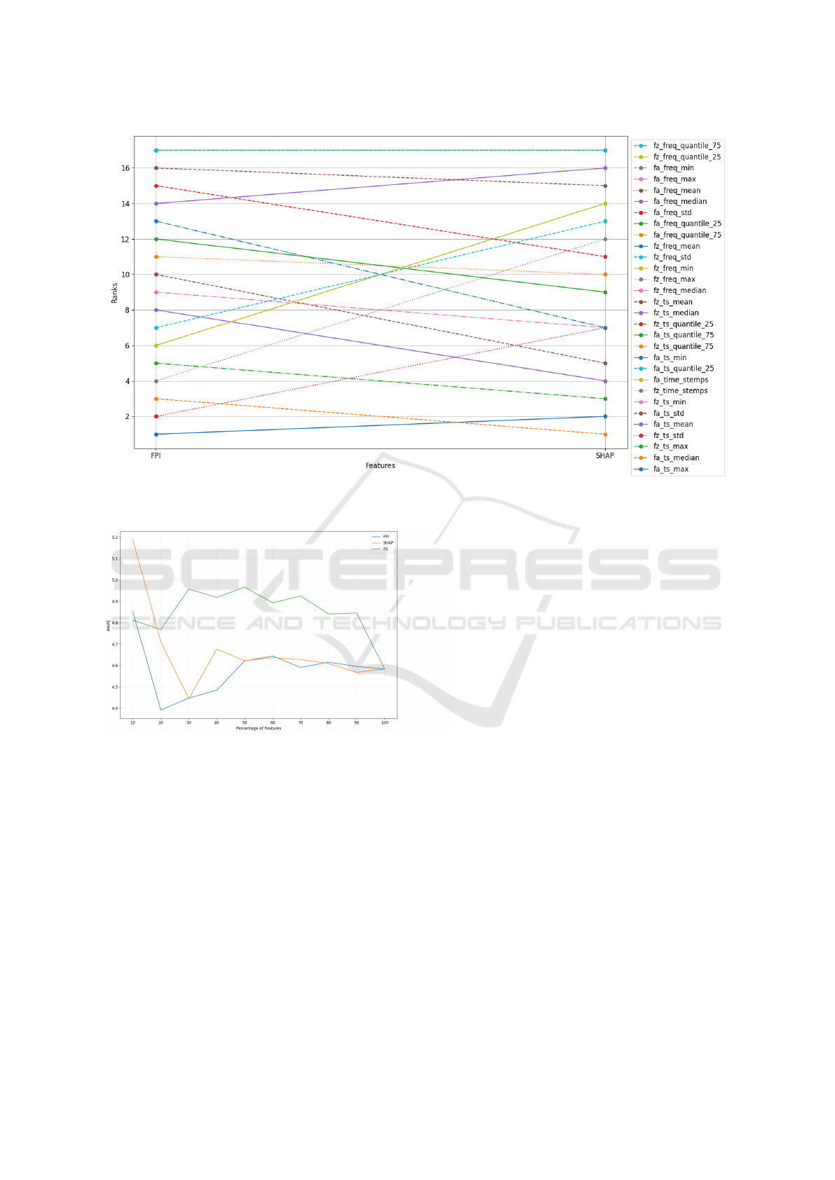
Figure 3: Visualization demonstrating the feature importance rank of Rdqmaxmean predictions, as elucidated by the feature

permutation importance permutation (FPI) and Shapley value (SHAP) method.

Figure 4: Using a different percentage of the most important

features based on the different methods for the Rdq predic-

tion. FS refers to feature selection.

top 20% of features deemed most critical (as deter-

mined by permutation importance), we enhanced the

MAPE from approximately 4.58 to 4.4.

5 DISCUSSION

Our case study shows the beneﬁt of explainable ML

techniques for quality prediction models in manufac-

turing. Explainability scores, as provided by the fea-

ture importance studied in our case study, allow to in-

terpret the results and determine the relevance of in-

dividual features for the predictive power of a model.

This interpretation can be utilized by human domain

experts for the analysis of the trained model and a

plausibility check, whether those features with high

importance are meaningful for the predictive task.

While it is known that ML models might reveal pre-

viously unknown relationships between input features

and the prediction target, this is a rather unlikely case

in our quality prediction setting. Instead, an overre-

liance on a speciﬁc feature can be an indicator for

learning a spurious correlation between an input and

the target, potentially caused by a lack of relevant data

in the small data regime. Explainability can, there-

fore, serve as an instrument for model validation and

human inspection.

Furthermore, the feature importance scores sup-

port the improvement of models, as demonstrated in

Section 4.4.3 by removing low-ranked features. Be-

sides improving the prediction accuracy of the actual

models, feature removal has additional beneﬁts for

deploying ML models for manufacturing quality pre-

diction. If the removed features relate to sensor data,

their removal also removes the necessity of frequently

reading and preprocessing that sensor, which reduces

the computational cost of making predictions. When

doing real-time quality prediction to detect potential

faults or deviations from the process plan during pro-

duction, minimizing the time needed to make a pre-

diction and increasing the frequency in which predic-

tions can be made is crucial.

In cases where the model development for quality

Enhancing Manufacturing Quality Prediction Models Through the Integration of Explainability Methods

903

prediction is considered during the prototyping phase

and construction of the manufacturing machine, the

relevance of features can inform the selection of phys-

ical sensors to be deployed on the machine. The pro-

totype machine is equipped with a larger set of sen-

sors, and only after evaluating the prediction models

is the ﬁnal set of relevant sensors determined.

Finally, besides the direct relation to the manu-

facturing case study, we see the beneﬁt of deploying

smaller, less complex, and ideally interpretable mod-

els (Breiman, 2001; Rudin et al., 2022). At the same

time, there is a trade-off between simplicity and ac-

curacy, referred to as the Occam dilemma (Breiman,

2001). The simpler a model is made, the less accurate

it gets. We see this in the case study from the error

difference between the simpler decision tree vs. the

more complex gradient-boosting trees or random for-

est. By applying explainability methods to reduce the

feature space, we again reduce the model complexity,

making the ﬁnal model more interpretable.

6 CONCLUSION

This study showcases the potential of combining ML

and explainability techniques to enhance the perfor-

mance of predictive models of surface quality in the

manufacturing sector, speciﬁcally in the context of

the milling process. Despite the limitations imposed

by data availability, our approach successfully lever-

ages less data-rich ML models, enhancing their efﬁ-

cacy through feature selection based on explainability

methods.

For future work, we are interested in extending the

application of explainability methods in ML models

to other manufacturing processes of our partners be-

yond milling to create a more comprehensive predic-

tive system. Additionally, utilizing these ML models

as digital twins for the corresponding physical ma-

chinery opens new avenues for employing parameter

optimization methods. This integration not only en-

hances the accuracy of the models but also provides

an opportunity for real-time ﬁne-tuning of machine

operations, thereby potentially improving efﬁciency

and reducing costs.

ACKNOWLEDGMENTS

This work is funded by the European Union under

grant agreement number 101091783 (MARS Project)

and as part of the Horizon Europe HORIZON-CL4-

2022-TWIN-TRANSITION-01-03.

REFERENCES

Bento, V., Kohler, M., Diaz, P., Mendoza, L., and Pacheco,

M. A. (2021). Improving deep learning performance

by using explainable artiﬁcial intelligence (xai) ap-

proaches. Discover Artiﬁcial Intelligence, 1:1–11.

Bins, J. and Draper, B. A. (2001). Feature selection from

huge feature sets. In Proceedings Eighth IEEE Inter-

national Conference on Computer Vision. ICCV 2001,

volume 2, pages 159–165. IEEE.

Breiman, L. (2001). Statistical Modeling: The Two Cul-

tures (with comments and a rejoinder by the author).

Statistical Science, 16(3):199–231.

Brusa, E., Cibrario, L., Delprete, C., and Di Maggio, L.

(2023). Explainable ai for machine fault diagno-

sis: Understanding features’ contribution in machine

learning models for industrial condition monitoring.

Applied Sciences, 13(4):20–38.

Chouhad, H., Mansori, M. E., Knoblauch, R., and Corleto,

C. (2021). Smart data driven defect detection method

for surface quality control in manufacturing. Meas.

Sci. Technol., 32(105403):16pp.

Fertig, A., Weigold, M., and Chen, Y. (2022). Machine

learning based quality prediction for milling processes

using internal machine tool data. Advances in Indus-

trial and Manufacturing Engineering, 4:100074.

Huang, N., Lu, G., and Xu, D. (2016). A permutation

importance-based feature selection method for short-

term electricity load forecasting using random forest.

Energies, 9(10):767.

Kummar, S. L. (2017). State of the art-intense review on

artiﬁcial intelligence systems application in process

planning and manufacturing. Engineering Applica-

tions of Artiﬁcial Intelligence, 65:294–329.

Kwon, H. J., Koo, H. I., and Cho, N. I. (2023). Un-

derstanding and explaining convolutional neural net-

works based on inverse approach. Cogn. Syst. Res.,

77:142–152.

Lampathaki, F., Agostinho, C., Glikman, Y., and Sesana, M.

(2021). Moving from ‘black box’ to ‘glass box’ arti-

ﬁcial intelligence in manufacturing with xmanai. In

2021 IEEE International Conference on Engineering,

Technology and Innovation (ICE/ITMC). Cardiff, UK.

Lozano-Murcia, C., Romero, F. P., Serrano-Guerrero, J.,

and Olivas, J. A. (2023). A comparison between

explainable machine learning methods for classiﬁca-

tion and regression problems in the actuarial context.

Mathematics, 11(14):3088.

Mokhtari Homami, R., Fadaei Tehrani, A., Mirzadeh, H.,

Movahedi, B., and Azimifar, F. (2014). Optimization

of turning process using artiﬁcial intelligence technol-

ogy. The International Journal of Advanced Manufac-

turing Technology, 70:1205–1217.

Mundada, V. and Narala, S. K. R. (2018). Optimization

of milling operations using artiﬁcial neural networks

(ann) and simulated annealing algorithm (saa). Mate-

rials Today: Proceedings, 5(2):4971–4985.

Myles, A. J., Feudale, R. N., Liu, Y., Woody, N. A., and

Brown, S. D. (2004). An introduction to decision tree

ICAART 2024 - 16th International Conference on Agents and Artiﬁcial Intelligence

904

modeling. Journal of Chemometrics: A Journal of the

Chemometrics Society, 18(6):275–285.

Nguyen, H. D. and Sakama, C. (2021). Feature learning by

least generalization. In ILP, volume 13191 of Lecture

Notes in Computer Science, pages 193–202. Springer.

Oreski, D., Oreski, S., and Klicek, B. (2017). Effects

of dataset characteristics on the performance of fea-

ture selection techniques. Applied Soft Computing,

52:109–119.

Otchere, D. A., Ganat, T. O. A., Ojero, J. O., Tackie-Otoo,

B. N., and Taki, M. Y. (2022). Application of gradient

boosting regression model for the evaluation of feature

selection techniques in improving reservoir character-

isation predictions. Journal of Petroleum Science and

Engineering, 208:109244.

Pawar, S., Bera, T., and Sangwan, K. (2021). Modelling of

energy consumption for milling of circular geometry.

Procedia CIRP, 98:470–475.

Pedregosa, F., Varoquaux, G., Gramfort, A., Michel, V.,

Thirion, B., Grisel, O., Blondel, M., Prettenhofer, P.,

Weiss, R., Dubourg, V., et al. (2011). Scikit-learn:

Machine learning in python. the Journal of machine

Learning research, 12:2825–2830.

Postel, M., Bugdayci, B., and Wegener, K. (2020). Ensem-

ble transfer learning for reﬁning stability predictions

in milling using experimental stability states. The In-

ternational Journal of Advanced Manufacturing Tech-

nology, 107:4123–4139.

Prasad, A. M., Iverson, L. R., and Liaw, A. (2006). Newer

classiﬁcation and regression tree techniques: bagging

and random forests for ecological prediction. Ecosys-

tems, 9:181–199.

Rudin, C., Chen, C., Chen, Z., Huang, H., Semenova, L.,

and Zhong, C. (2022). Interpretable machine learn-

ing: Fundamental principles and 10 grand challenges.

Statistics Surveys, 16:1–85.

Schorr, S., Moller, M., Heib, J., Fang, S., and Bahre, D.

(2020). Quality prediction of reamed bores based on

process data and machine learning algorithm: A con-

tribution to a more sustainable manufacturing. Proce-

dia Manufacturing, 43:519–526.

Senoner, J., Netland, T. H., and Feuerriegel, S. (2022). Us-

ing explainable artiﬁcial intelligence to improve pro-

cess quality: Evidence from semiconductor manufac-

turing. Manag. Sci., 68(8):5704–5723.

Soﬁanidis, G., Ro

zanec, J. M., Mladeni

c, D., and Kyriazis,

D. (2021). A review of explainable artiﬁcial intelli-

gence in manufacturing.

Sun, H., Servadei, L., Feng, H., Stephan, M., Santra, A., and

Wille, R. (2022). Utilizing explainable ai for improv-

ing the performance of neural networks. In 2022 21st

IEEE International Conference on Machine Learning

and Applications (ICMLA), pages 1775–1782. IEEE.

Sundararajan, M. and Najmi, A. (2020). The many shapley

values for model explanation. In International confer-

ence on machine learning, pages 9269–9278. PMLR.

Venkatesh, B. and Anuradha, J. (2019). A review of feature

selection and its methods. Cybernetics and informa-

tion technologies, 19(1):3–26.

Yoo, S. and Kang, N. (2021). Explainable artiﬁcial intelli-

gence for manufacturing cost estimation and machin-

ing feature visualization. Expert Systems with Appli-

cations, 183.

Enhancing Manufacturing Quality Prediction Models Through the Integration of Explainability Methods

905