An Insight Into Neurodegeneration: Harnessing Functional MRI

Connectivity in the Diagnosis of Mild Cognitive Impairment

Shuning Han

1,2 a

, Zhe Sun

2,3 b

Kanhao Zhao

4 c

, Feng Duan

5 d

, Cesar F. Caiafa

6 e

Yu Zhang

4,7 f

and Jordi Sol

e-Casals

1,8 g

Data and Signal Processing Research Group, University of Vic-Central University of Catalonia, Vic, 08500, Catalonia,

Spain

Image Processing Research Group, RIKEN Center for Advanced Photonics, Riken, Wako-Shi, Saitama, Japan

Faculty of Health Data Science, Juntendo University, Urayasu, Chiba, Japan

Department of Bioengineering, Lehigh University, Bethlehem, PA 18015, U.S.A.

Tianjin Key Laboratory of Brain Science and Intelligent Rehabilitation, Nankai University, Tianjin, China

Instituto Argentino de Radioastronom

ıa-CCT La Plata, CONICET/ CIC-PBA/ UNLP, V. Elisa 1894, Argentina

Department of Electrical and Computer Engineering, Lehigh University, Bethlehem, PA 18015, U.S.A.

Department of Psychiatry, University of Cambridge, Cambridge CB20SZ, U.K.

ﬁ

Keywords:

Alzheimer’s Disease, Mild Cognitive Impairment, Graph Convolutional Network, Functional Magnetic

Resonance Imaging Analysis, Functional Connectivity.

Abstract:

Alzheimer’s disease is a progressive form of memory loss that worsens over time. Detecting it early, when

memory issues are mild, is crucial for effective interventions. Recent advancements in computer technology,

speciﬁcally Graph Convolutional Networks (GCNs), have proven to be powerful tools for analyzing Magnetic

Resonance Imaging (MRI) data comprehensively. In this study, we developed a GCN framework for diagnos-

ing mild cognitive impairment (MCI) by examining the functional connectivity (FC) derived from resting-state

functional MRI (rfMRI) data. Our research systematically explored various types and processing methods of

FC, evaluating their performance on the OASIS-3 dataset. The experimental results revealed several key ﬁnd-

ings. On the one hand, the proposed GCN exhibited signiﬁcantly superior performance over both the baseline

GCN and the Support Vector Machine (SVM) models, with statistically signiﬁcant differences. It attained

the highest average accuracy of 80.3% and a peak accuracy of 88.2%. On the other hand, the GCN frame-

work obtained using individual FCs showed overall slightly better performance than the one using global FCs.

However, it is important to note that GCNs using global networks with appropriate connectivity can achieve

comparable or even better performance than individual networks in certain cases. Finally, our results also

indicate that the connectivity within speciﬁc brain regions, such as VIS, DMN, SMN, VAN, and FPC, may

play a more signiﬁcant role in GCN-based MRI classiﬁcation for MCI diagnosis. These ﬁndings signiﬁcantly

contribute to the understanding of neurodegenerative disorders and offer valuable insights into the diverse ap-

plications of GCNs in brain analysis and disease detection.

https://orcid.org/0009-0004-0792-5484

https://orcid.org/0000-0002-6531-0769

https://orcid.org/0000-0002-2955-0917

https://orcid.org/0000-0002-2179-2460

https://orcid.org/0000-0001-5437-6095

https://orcid.org/0000-0003-4087-6544

https://orcid.org/0000-0002-6534-1979

1 INTRODUCTION

Alzheimer’s disease (AD) is a progressive neurode-

generative dementia Srivastava et al. (2021). The typ-

ical progression of AD comprises three stages: (early)

mild cognitive impairment (MCI), moderate demen-

tia, and severe dementia. Detecting patients in the

MCI stage is crucial, as it facilitates the implemen-

tation of effective interventions to prevent further de-

terioration of dementia.

656

Han, S., Sun, Z., Zhao, K., Duan, F., Caiafa, C., Zhang, Y. and Solé-Casals, J.

An Insight Into Neurodegeneration: Harnessing Functional MRI Connectivity in the Diagnosis of Mild Cognitive Impairment.

DOI: 10.5220/0012414600003657

Paper published under CC license (CC BY-NC-ND 4.0)

In Proceedings of the 17th International Joint Conference on Biomedical Engineering Systems and Technologies (BIOSTEC 2024) - Volume 1, pages 656-666

ISBN: 978-989-758-688-0; ISSN: 2184-4305

Due to the intricate nature of data from various

imaging modalities and the organisational complex-

ity of the human brain network, promising advances

have been observed in modelling the interactions be-

tween various brain regions. This progress is in part

due to new learning techniques that rely on graphs

derived from image data, apply graph regularisations

to the data, and employ graph embedding to repre-

sent graphs derived from recorded data. These meth-

ods show potential for capturing the fusion of infor-

mation between networks from different brain imag-

ing modalities, modelling latent spaces within high-

dimensional brain networks, and quantifying neuro-

biomarkers based on topological features (Liu et al.,

2022).

In recent years, research on magnetic resonance

imaging (MRI) has signiﬁcantly contributed to our

comprehension of neuropathological mechanisms un-

derlying dementia and its clinical diagnosis (Chan-

dra et al., 2019). Functional MRI (fMRI) furnishes

valuable insights with a relatively high spatial reso-

lution (2mm isotropic) and medium temporal resolu-

tion (minutes) (Liu et al., 2015). fMRI can be cat-

egorized into two types: task-evoked fMRI (tfMRI),

collected while the subject is engaged in tasks, and

resting-state fMRI (rfMRI), collected during periods

of rest. Even in the resting state, spatial patterns of

spontaneous neural activities and metabolism persist

in the brain. The functional connectivity (FC) be-

tween various brain regions can be inferred (Bi et al.,

2020). FC serves as a reﬂection of the brain’s func-

tional organization, and alterations in it are believed

to be associated with psychiatric disorders (Bullmore

and Sporns, 2009).

Recently, the integration of graph theory and ma-

chine learning techniques has found extensive appli-

cation in neuroscience for the analysis of the brain

and the detection of diseases (Bi et al., 2020). A novel

domain of geometric deep learning, graph neural net-

works (GNNs), has emerged, which offers the capa-

bility to effectively process signals within the non-

Euclidean geometry of graphs. Notably, an increas-

ing number of GNNs have been introduced and em-

ployed in the analysis of brain MRI and the detec-

tion of disorders (Scarselli et al., 2008). For instance,

a graph empirical mode decomposition-based data

augmentation was presented in (Chen et al., 2022)

to generate more samples in small datasets. Parisot

et al. (2017) introduced the graph convolution net-

work (GCN) combining fMRI with non-imaging data

for brain analysis and disease diagnosis. Wang et al.

(2021) presented a connectivity based GCN architec-

ture for fMRI analysis and applied it to classiﬁca-

tion of autistic patients from normal controls (NCs).

Tang et al. (2022) proposed a contrastive learning

framework with an interpretable hierarchical signed

graph representation learning model for brain func-

tional network mining. Qu et al. (2023) proposed a

univariate neurodegeneration biomarker based GCN

semi-supervised classiﬁcation framework. Neverthe-

less, there has been insufﬁcient research dedicated to

assessing the inﬂuence of various FC on brain analy-

sis results. Moreover, the performance of GCN mod-

els in MCI detection still falls short of expectations.

Considering the points mentioned above, this

study introduces a state-of-art approach in the realm

of neurodegeneration detection using fMRI data. The

key highlights of this research are as follows:

A Novel FC Based GCN Framework for MCI

Fetection: We have designed a novel FC based GCN

framework for binary classiﬁcations utilizing rfMRI

data. The GCN framework is applied for the diagnosis

of MCI by classifying the MCI from NCs.

Impact of Different Types of FC: This study

places special emphasis on understanding the effects

of different FC types and processing methods on the

GCN framework’s performance. In this paper, FC is

regarded as a graph and is considered from two as-

pects: On one side, we compare the difference of us-

ing the global FC matrix obtained from the training

data versus the individual speciﬁc FC matrices of each

rfMRI data. On the other side, we employ different

processing methods for the FC matrices, and obtain

the k nearest neighbor (k-NN) graph and the thresh-

old graph.

An Insight Into Neurodegeneration: The study

delves deeply into the analysis of brain networks in-

cluding self-network and between-network connec-

tivity. This perspective enhances the clinical rele-

vance of neurodegeneration and impact of this study’s

ﬁndings.

The remainder of this paper is structured as fol-

lows: Section 2 provides an overview of the dataset

and methods employed. In Section 3, we present the

analysis results, which are subsequently discussed in

Section 4. Finally, Section 5 concludes this study.

2 MATERIALS AND METHODS

In this section, we initially introduce the dataset for

classiﬁcation and elucidate the label assignment pro-

cess. Following that, we detail the fMRI acquisi-

tion and preprocessing methods, generation of diverse

FC, and ﬁnally the proposed GCN framework and the

baseline methods used for comparison.

An Insight Into Neurodegeneration: Harnessing Functional MRI Connectivity in the Diagnosis of Mild Cognitive Impairment

657

2.1 Data

We utilize longitudinal rfMRI series for analysis, cat-

egorizing them into NC and MCI based on the rele-

vant clinical assessments of the participants.

2.1.1 OASIS-3 Dataset

We employ the dataset from the Open Access Series

of Imaging Studies (OASIS)-3 (LaMontagne et al.,

2019) (https://www.oasis-brains.org) to vali-

date our proposed GCN framework. The dataset in-

cludes longitudinal fMRI, neuropsychological testing

and clinical information for 1098 participants. The

clinical dementia rating (CDR) scale is utilized to

evaluate the dementia status within the clinical data

of OASIS-3: CDR 0 denotes normal cognitive func-

tion, CDR 0.5 indicates very mild impairment, CDR

1 signiﬁes mild impairment, and CDR 2 reﬂects mod-

erate dementia. All participants were required to have

a CDR ≤ 1 in the most recent clinical core assess-

ment, and once a participant reached CDR 2, they

were no longer eligible for continued participation in

the study.

2.1.2 MRI Scans Labelling

MRI scans can be labeled based onNotably, associ-

ated CDR values. Notably, clinical assessments were

performed on different days from the neural imaging

scans, and the time gap between the MRI scan and

clinical assessment may exceed one year in the lon-

gitudinal OASIS-3 dataset. In this study, MRI scans

are classiﬁed into two groups: NC and MCI based

on CDR values. An MRI scan is labeled as NC, if

all recorded clinical assessment results for the corre-

sponding subject are CDR = 0; an MRI scan is labeled

as MCI, if both preceding and subsequent clinical as-

sessment show CDR ≥ 0.5. For the purpose of main-

taining data balance, 503 NC and MCI rfMRI samples

are used for MCI detection, respectively.

2.2 Methods

This part provides a comprehensive exposition on the

fMRI acquisition and pre-processing methods, along

with the various FC processing methods. Following

that, we delve into a detailed description of the pro-

posed GCN framework and the baselines. Finally,

we present the speciﬁc conﬁgurations of the proposed

GCN framework.

2.2.1 fMRI Acquisition and Preprocessing

The fMRI data for each subject in each run were ac-

quired in resting state for 6 min (164 volumes) uti-

lizing 16-channel head coil in the scanners. The

acquired rfMRI data underwent preprocessing us-

ing the fMRIPrep pipeline (Esteban et al., 2019).

The T1-weighted (T1w) image underwent intensity

correction, skull-stripping, and spatial normaliza-

tion through nonlinear registration (Avants et al.,

2008). Employing FSL, brain features such as

cerebrospinal ﬂuid, white matter, and grey matter

were segmented from the reference, brain-extracted

T1 weighted image (Zhang et al., 2000). The

ﬁeldmap information was used to correct distortion

in low-frequency and high-frequency components of

ﬁeldmap. Subsequently, a corrected echo-planar

imaging reference was obtained from a more ac-

curate co-registration with the anatomical reference.

The blood-oxygenation-level-dependent (BOLD) ref-

erence was then transformed to the T1-weighted im-

age with a boundary-based registration method, con-

ﬁgured with nine degrees of freedom to account for

distortion remaining in the BOLD reference (Greve

and Fischl, 2009). Head-motion parameters were es-

timated with MCFLIRT (FSL). BOLD signals were

slice-time corrected and resampled onto the partic-

ipant’s original space with head-motion correction,

susceptibility distortion’s correction, and then resam-

pled into standard space, generating a preprocessed

BOLD run in MNI152NLin2009cAsym space. Auto-

matic removal of motion artifacts using independent

component analysis (ICA-AROMA) (Pruim et al.,

2015) was performed on the preprocessed BOLD

time-series on MNI space after removal of non-

steady-state volumes and spatial smoothing.

2.2.2 FC Construction

The brain FC can be derived from rfMRI and repre-

sented as graphs, capturing the statistical time-series

correlations between brain regions of interest (ROIs).

The preprocessed BOLD-level rfMRI series are aver-

aged into 100 ROIs deﬁned by Schaefer atlas (Schae-

fer et al., 2018) and subsequently standardized using

z-score. Ultimately, the dimension of each fMRI ses-

sion is 164 × 100 (100 regions with a length of 164

time samples each). To construct the FC matrices

for ROIs, the Pearson correlation coefﬁcient (PCC) is

computed between the fMRI time series of every pair

of brain regions. Notably, in this study, the diagonal

elements of the FC matrices are uniformly set to 0.

There are 100 ROIs, resulting in an FC matrix with a

shape of 100 × 100.

In this paper, we analyse the impact of various

types of FC on prediction results, as depicted in Fig-

ure 1. The divergence in FC manifests in two dimen-

sions: one is the different FC matrices, individual spe-

ciﬁc FC matrices obtained from each fMRI data vs.

BIOSIGNALS 2024 - 17th International Conference on Bio-inspired Systems and Signal Processing

658

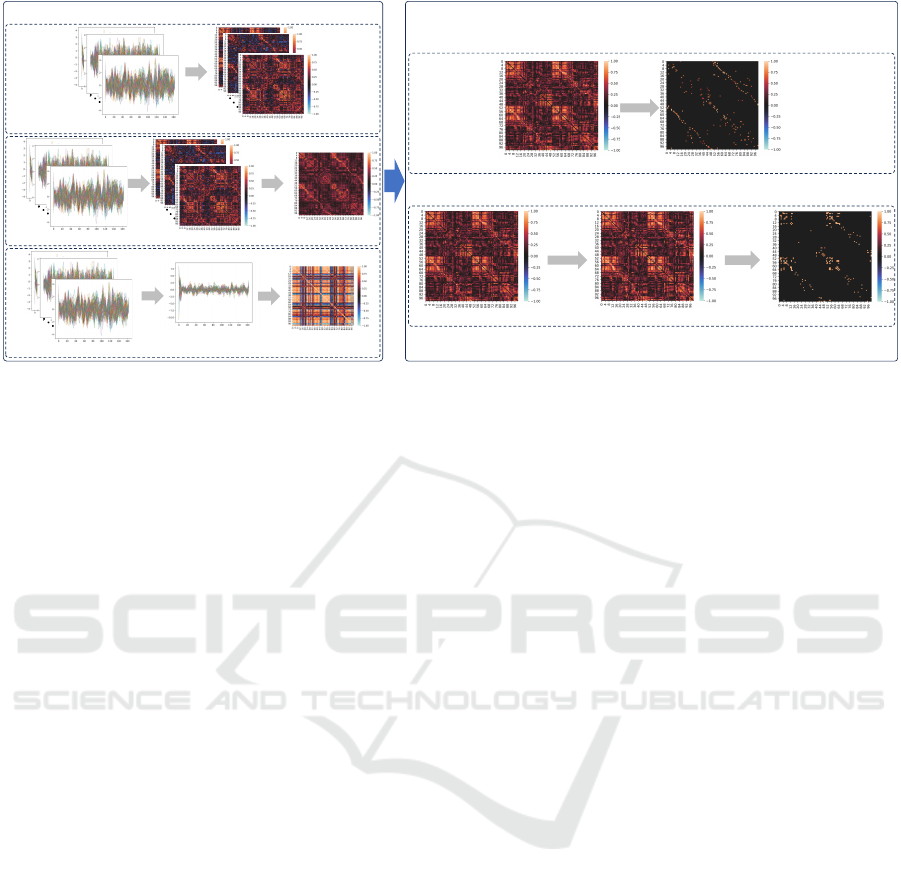
FC-of-avgROI

Average

PCC

avgFC

PCC

k-NN

Absolute FC k-NN graph

Absolute FC Threshold graphNAFC

Approaches for Obtaining Different Types of FC

Normalize

Different Graph Processing Methods

Threshold

Average

fMRI samples

Training fMRI samples

Individual specific FC

Training fMRI samples

Figure 1: FC construction. Left part: a. Approach for individual speciﬁc FC; b. Approach for global FC-of-avgROI; c.

Approach for global avgFC; Right part: d. Method for k-NN graph; e. Method for threshold graph.

global FC matrix obtained from the training data for

both training and testing data; the other is the different

processing methods employed to derive the FC matri-

ces. In Han et al. (2024), an extensive and compre-

hensive analysis is carried out, delving into a wider

range of aspects to provide a global understanding.

This extended analysis includes the examination of

two additional forms of FC, namely top-p and the p-

MST (Minimum Spanning Tree). The exploration of

these speciﬁc types of FC aims to capture a more de-

tailed perspective of the intricate network dynamics

within the brain. In addition, the research extends its

focus by addressing the classiﬁcation of at-risk de-

mentia versus normal control subjects. This compar-

ative analysis offers valuable insights into the unique

neural signatures associated with this particular con-

dition when contrasted with the normal control group.

• Obtain global FC matrix from training data

Individual speciﬁc FC matrices can be derived

from each fMRI data by directly computing PCC, as

illustrated in Figure 1a. While, a global FC matrix

for both training and testing fMRI samples is derived

from training samples using distinct approaches. In

the ﬁrst approach for global FC, the FC-of-avgROI

matrix is obtained from the standardized average data

of the training fMRI samples, as illustrated in Fig-

ure 1b. In the second approach, we regard the average

PCC of all PCC matrices from the training fMRI sam-

ples, denoted as avgFC, as the global FC matrix, as

shown in Figure 1c.

Special to note is that: (i) matrix averaging oper-

ations are performed across subjects; (ii) the global

avgFC was also utilized in the baseline GCN; (iii) the

ﬁnal obtained FC matrices are further processed using

the methods in “Different graph processing meth-

ods”, depicted in the right part of Figure 1.

• Different graph processing methods

To investigate the impact of different graph types

on the classiﬁcation results of GCN, we employ vari-

ous processing methods to individual or global FC, as

shown in the right part of Figure 1. In the ﬁrst method,

we take the k largest values in each row of the absolute

FC matrix as the k-NN graph, as shown in Figure 1d.

In the second method, we normalize the absolute FC

values to the range [0− 1] for consistent thresholding,

denoted as the normalized absolute FC (NAFC), and

then the thresholding is applied on the NAFC matrix

(denoted as threshold graph), as illustrated in Figure

1e.

2.2.3 Graph Convolutional Network (GCN)

Graphs (Zhou et al., 2020) represent a non-Euclidean

data structure comprising nodes and edges, where

nodes denote objects and edges signify relation-

ships between these objects. Brain FC can be

modeled as graphs, with nodes representing ROIs

and edges corresponding to activity correlations be-

tween these ROIs (Hanik et al., 2022; Sporns et al.,

2005; Suprano, 2019). GCNs (Scarselli et al., 2008;

Micheli, 2009) have gained widespread popularity

in machine learning for graph analysis, owing to

their persuasive performance. The GCN architec-

tures effectively integrate node features and graph

topology to construct distributed node representations

with graph convolutional layers (GCLs) (Errica et al.,

2020). In this work, we introduce a novel GCN frame-

work for binary classiﬁcation of fMRI data, where the

fMRI time series of brain ROIs are directly regarded

as the node features and the FC serves as the graph

topology.

An Insight Into Neurodegeneration: Harnessing Functional MRI Connectivity in the Diagnosis of Mild Cognitive Impairment

659

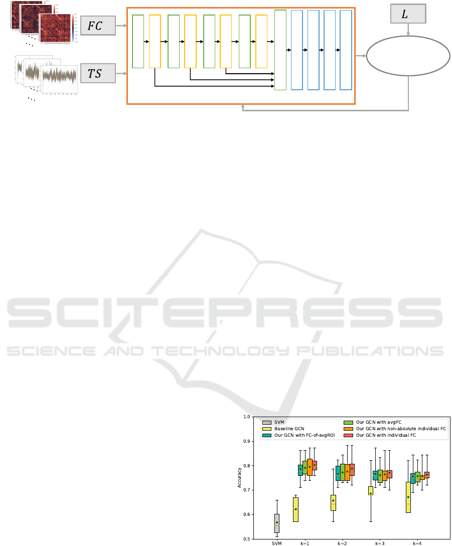
• The Proposed GCN

The proposed GCN framework is implemented

using the Pytorch Geometric (PyG) library (Fey and

Lenssen, 2019). This library encompasses a vari-

ety of GNN models and graph preprocessing meth-

ods to easily build and train GNNs. The designed

GCN framework, illustrated in Figure 2, comprises

ﬁve GCLs based on GraphConv (Morris et al., 2019).

The nonlinear activation function Rectiﬁed Linear

Unit (ReLU) (Nair and Hinton, 2010) layer deﬁned

as f (x) = max(0, x) follows after each of the ﬁrst 4

GCLs. The input of the last GCL layer is the outputs

of the ﬁrst 4 layers. The ﬁfth GCL includes a batch

normalization layer, enhancing the speed and stabil-

ity of the GCN framework. Subsequently, the global

mean pool or global average pool is followed to avoid

overﬁtting and enhance the robustness of the frame-

work. To further prevent overﬁtting, a dropout layer

is implemented, randomly setting output data to zero

with a speciﬁed probability.

In the presented GCN framework, the optimiza-

tion is carried out using the Adam algorithm (Kingma

and Ba, 2015), and the loss function employed is the

cross-entropy loss. The proposed GCN framework

is applied for two types of classiﬁcation: one with

global FC and the other with individual FC. For the

classiﬁcation with individual FC, as illustrated in Fig-

ure 2, the inputs consist of individual time series of

ROIs with corresponding FC and labels. While, in the

classiﬁcation with global FC, the inputs of the GCN

framework are individual time series of ROIs with the

same global FC and labels of each sample.

• Baselines

For the purpose of comparison, we establish

two baselines: the Support Vector Machine (SVM)

employing the radial basis function (RBF) kernel

(Burges, 1998), and the GCN architecture for fMRI

analysis developed by Wang et al. (Wang et al., 2021)

in 2021.

The baseline GCN architecture using avgFC con-

sisted of 5 convolutional layers, one recurrent neu-

ral network (RNN) layer and a Softmax layer. In the

original study, the GCN was applied for autism spec-

trum disorder (ASD) classiﬁcation, attaining the best

average accuracy of 70.7% (max 79.0%, min 66.7%)

when k = 3 (among 3, 5, 10, and 20) using 10-fold

cross validation.

2.2.4 Conﬁgurations

We reimplement the baseline GCN architecture and

apply it to the OASIS-3 dataset using all recom-

mended parameters from the original paper. In the

current study, a 10-fold cross validation strategy is

adopted to evaluate the performance of the GCN

framework which is set to be the same when apply-

ing the baseline GCN to OASIS-3 dataset.

Code of the proposed GCN framework is imple-

mented based on Python, and the GCN structure is re-

alized by PyTorch based on PyG. In our experiment,

the output dimension of each convolutional layer is

128; the learning rate is set to 0.001; the dropout rate

is set to 0.5; and the model is trained for 100 epochs

with a batch size of 8.

To assess the impact of variations in the FC ma-

trix on the outcomes, we varied the number of nearest

neighbors k (1, 2, 3, and 4) and the threshold value

(0.7, 0.8, 0.9, 0.95, and 0.99) for FC matrix process-

ing. To evaluate the signiﬁcant differences in clas-

siﬁcation results between the proposed GCN and the

baseline GCN, as well as those between GCN with

different types of FC, the independent t-test method

was employed in this study. The brain networks of

different global graphs in one fold are visualized with

Brainnet viewer (Xia et al., 2013). The brain net-

works are grouped into seven canonical functional

networks deﬁned by the 7 Yeo networks (Buckner

et al., 2011): visual network (VIS), somatomotor net-

work (SMN), dorsal attention network (DAN), ven-

tral attention network (VAN), limbic network (LIM),

frontoparietal control network (FPC), default mode

network (DMN).

3 RESULTS

As mentioned earlier, to better understand the impact

of different FC, the proposed GCN utilizes the graphs

of global FC (avgFC or FC-of-avgROI) or individual

FC, and then the graphs are processed as k-NN graph

and threshold graph, respectively. In this section,

we provide the classiﬁcation results for MCI vs. NC

using GCN with k-NN graphs or threshold graph.

3.1 Results with k-NN Graph

We implement the MCI vs. NC classiﬁcation of the

proposed GCN with k-NN graphs obtained from

individual FC, non-absolute individual FC, global

FC of avgFC and FC-of-avgROI. Especially, we

also utilize the non-absolute individual FC here to

demonstrate the superiority of GCN with absolute FC

over that with non-absolute FC. It should be noted

that absolute FC are used as the default in this article.

We compare the performance of our proposed GCN

with the baseline GCN framework and SVM method.

The experimental results are shown in Figure 3,

which illustrates that:

BIOSIGNALS 2024 - 17th International Conference on Bio-inspired Systems and Signal Processing

660



𝑇𝑆



Cross-entropy

loss

𝑇𝑆



𝐹𝐶





𝑇𝑆



𝐹𝐶



𝐹𝐶



GraphConv

ReLU

GraphConv

ReLU

GraphConv

ReLU

GraphConv

ReLU

BatchNorm

Global Mean Pool

Dropout

Linear

GNN

Figure 2: GCN classiﬁcation with individual FC. T S

denotes the ith individual time series of ROIs; FC

and L

denote the

corresponding ith individual FC and label. In the classiﬁcation with global FC, we utilize one same global FC for each

individual time series of ROI.

1) The proposed GCN outperforms both the

baseline GCN (best average accuracy of 68.6% when

k = 3) and SVM (average accuracy of 56.8%) in

terms of accuracy. The t-test outcomes in Table 1

show signiﬁcant differences between the results of

proposed GCN and the baseline GCN with different

values of k at the 5% signiﬁcance level. Our proposed

GCN with k-NN graphs achieves the best average

accuracy of 80.3% (max 87.3%, min 76.0%) with

absolute-individual FC when k = 1.

2) The proposed GCN with k-NN graphs exhibits

differently compared to the baseline GCN. While the

accuracy of the baseline GCN increases as k increases

and achieves the best average accuracy at k = 3 (the

same as in ASD classiﬁcation in the baseline paper),

our proposed GCN’s performance with individual or

global FC declines as k increases.

3) The proposed GCN with absolute individual

FC demonstrates a slight performance improvement

compared to its counterpart with non-absolute indi-

vidual FC.

4) Our proposed GCN with individual FC per-

forms slightly better than that with global FC. The

use of global avgFC or FC-of-avgROI exhibits neg-

ligible differences for the proposed GCN with k-NN

graphs.Besides, the t-test results in Table 2 indicate

that there are no signiﬁcant differences between the

outcomes of the individual and the two types of global

FC across various values of k at the 5% signiﬁcance

level.

Brain networks of k-NN graphs of avgFC or FC-

of-avgROI are displayed as Figure 4. It is important

to note that the k-NN graphs are non-symmetrical

matrices and cannot guarantee full connectivity. In

this ﬁgure, there are only 50 and 45 edges in avgFC

and FC-of-avgROI as k = 1, respectively. From the

brain networks, it can be observed that:

1) Increasing k leads to more edges in both avgFC

and FC-of-avgROI brain networks.

This highlights an important ﬁnding that ex-

cessive connectivity can have a detrimental effect

on improving classiﬁcation performance, which is

evidenced by the diminishing performance results as

the number of connectivity (k) increases.

2) The brain networks of k-NN avgFC and

FC-of-avgROI show little difference for each value

of k, which can explain the negligible difference of

the accuracy between avgFC and FC-of-avgROI with

the same k.

3) The brain networks of avgFC involve a slightly

larger number of ROIs than FC-of-avgROI when k =

1, 2, and the average accuracy of GCN with avgFC

are marginally higher than that of GCN with FC-of-

avgROI. This ﬁnding illustrates that graphs involving

a greater number of nodes may contain more valuable

information for GCN classiﬁcation.

Figure 3: MCI vs. NC results of the proposed GCN frame-

work with k-NN graph. The black dot in the box presents

the average value in the 10-fold cross validation results.

An Insight Into Neurodegeneration: Harnessing Functional MRI Connectivity in the Diagnosis of Mild Cognitive Impairment

661

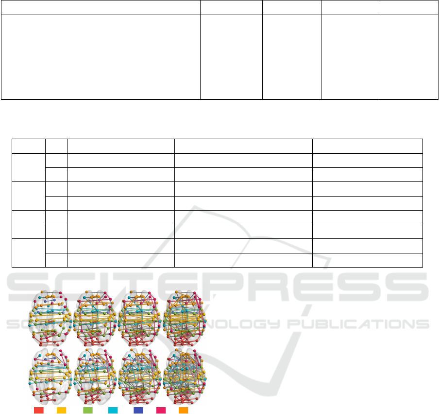
Table 1: The probability results in t-test between baseline methods and our proposed GCNs with k-NN graph.

t − test k = 1 k = 2 k = 3 k = 4

Baseline GCN vs. our GCN with individual FC 1.72 × 10

−8

5.19 × 10

−5

3.51 × 10

−3

2.97 × 10

−3

Baseline GCN vs. our GCN with avgFC 7.10 × 10

−8

1.20 × 10

−4

6.48 × 10

−3

4.43 × 10

−3

Baseline GCN vs. our GCN with FC-of-avgROI 3.32 × 10

−7

1.99 × 10

−4

5.43 × 10

−3

7.35 × 10

−3

SVM vs. our GCN with individual FC 4.47 × 10

−10

1.04 × 10

−8

1.87 × 10

−8

9.00 × 10

−9

SVM vs. our GCN with avgFC 1.54 × 10

−9

1.19 × 10

−8

1.80 × 10

−8

9.84 × 10

−9

SVM vs. our GCN with FC-of-avgROI 6.96 × 10

−9

1.73 × 10

−8

2.78 × 10

−8

5.73 × 10

−8

Table 2: t-test results between our proposed GCNs with k-NN graph of different types (individual, avgFC, FC-of-avgROI).

P denotes the probability and CI denotes the conﬁdence interval in the t-test.

t-test avgFC vs. individual FC FC-of-avgROI vs. individual FC FC-of-avgROI vs. avgFC

k = 1

P 0.47 0.36 0.79

CI [-0.046,0.022] [-0.055,0.021] [-0.044,0.034]

k = 2

P 0.45 0.30 0.76

CI [-0.059,0.027] [-0.064,0.021] [-0.045,0.034]

k = 3

P 0.61 0.81 0.80

CI [-0.049,0.030] [-0.047,0.037] [-0.035,0.045]

k = 4

P 0.70 0.70 0.95

CI [-0.038,0.026] [-0.045,0.031] [-0.038,0.036]

k = 1 k = 2 k = 3 k = 4

avgFC

FC-of-

avgROI

VIS SMN DAN VAN LIM FPC DMN

Figure 4: The brain networks of k-NN avgFC or FC-of-

avgROI. The seven-colored nodes are indicative of seven

grouped networks (VIS, SMN, DAN, VAN, LIM, FPC,

DMN), while color-coded links denote self-network con-

nectivity and grey links denote the between-network con-

nectivity.

3.2 Results with Threshold Graph

The MCI vs. NC classiﬁcation performances of the

proposed GCN with threshold graph derived from

individual FC, global FC of avgFC or FC-of-avgROI

are reported in Figure 5. It can be observed that:

1) As the threshold value increases, the accuracy

of GCN with FC-of-avgROI performs differently

from that of GCN with individual FC or avgFC. The

t-test outcomes in Table 3 show signiﬁcant differ-

ences between the results of the FC-of-avgROI and

individual FC or avgFC with threshold = 0.7, 0.8, 0.9

or 0.95 at the 5% signiﬁcance level

2) The average accuracy of GCN with FC-

of-avgROI graphs are notably lower compared

to that of GCN with individual FC or avgFC as

threshold ≤ 0.95, and then exhibits a signiﬁcant rise

when the threshold reaches 0.99.

3) The average accuracy of GCN with individual

and avgFC graphs show a gradual increase and attain

an optimal average accuracy at threshold = 0.95

and threshold = 0.90, respectively. Nonetheless,

the accuracy of both decrease when threshold = 0.99.

4) In some cases (avgFC with all threshold val-

ues and FC-of-avgROI as threshold = 0.99), the GCN

with global FC achieves comparable or even supe-

rior performance compared with GCN using individ-

ual FC. Moreover, the t-test outcomes in Table 3 indi-

cate that there are no signiﬁcant differences between

the results of the individual and avgFC across vari-

ous threshold values, and between the results of the

individual and FC-of-avgROI as threshold = 0.99 at

the 5% signiﬁcance level. Overall, the proposed GCN

with threshold graphs achieves the best average accu-

BIOSIGNALS 2024 - 17th International Conference on Bio-inspired Systems and Signal Processing

662

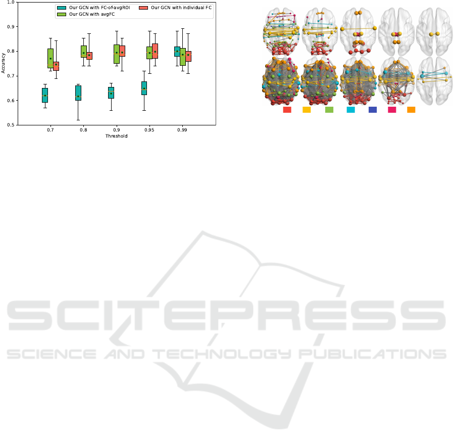
Figure 5: MCI vs. NC results of the proposed GCN frame-

work with threshold graph.

racy of 80.0% (max 88.2%, min 74.0%) with FC-of-

avgROI graphs when threshold = 0.99.

The brain networks of avgFC and FC-of-avgROI

with different threshold values are displayed in

Figure 6. It can be observed that:

1) Increasing threshold results in fewer edges in

both networks. However, FC-of-avgROI contains

much more edges than avgFC when threshold > 0.7.

When few edges remain in the graph, there are

self-network edges of SMN, DMN, FPC, and VIS

in avgFC (threshold = 0.9 or threshold = 0.95);

while, there are both self-network and between-

network edges of SMN and VAN in FC-of-avgROI

(threshold = 0.99).

2) The GCN with global FC that have very

few edges in the graph obtained a higher average

accuracy, which emphasizes the observation in k-NN

graphs that excessive connectivity can negatively

affect classiﬁcation performance.

3) The slight decrease in average GCN accu-

racy with avgFC when there is only one edge left

(threshold = 0.99) shows that a minimum number of

edge information can cause a slight decrease in accu-

racy, although the ROI series contain a large amount

of information. Furthermore, with suitable connec-

tivity, the GCN with global FC can achieve compa-

rable or superior performance compared with GCN

with individual FC. These ﬁndings highlight the sig-

niﬁcance of suitable edge information for achieving

performance, rather than the threshold itself.

4 DISCUSSION

In this study, we developed an FC based GCN frame-

work for fMRI binary classiﬁcations to detect MCI

thr = 0.7 thr = 0.8 thr = 0.9 thr = 0.95 thr = 0.99

avgFC

FC-of-

avgROI

VIS SMN DAN VAN LIM FPC DMN

Figure 6: The brain networks of threshold avgFC or FC-of-

avgROI. The size of nodes reﬂects the degree of the graph,

and the nodes in k-NN graph have the same size. Other

annotations are identical to Figure 4.

from NCs on the longitudinal OASIS-3 dataset. Be-

sides, we explored the impact of different types and

processing methods of FC on the GCN classiﬁcation

performance.

The results of our experiments revealed several

important ﬁndings. First, our proposed GCN signiﬁ-

cantly outperformed both the baseline GCN and SVM

in terms of accuracy, indicating its effectiveness for

MCI diagnosis. The proposed GCN achieved the best

average accuracy of 80.3% (11.7 % higher than the

baseline GCN and 23.5% higher than SVM) and the

highest accuracy of 88.2%. This highlights the poten-

tial of deep learning techniques, speciﬁcally the GCN

framework, for analyzing rfMRI data and detecting

neurodegenerative disorders.

Second, we compared the effects of different types

of FC utilized in the GCN. The proposed GCN with

absolute individual FC performed slightly better than

non-absolute individual FC. In this study, we found

that the GCN framework with individual FC per-

formed slightly better than that with global FC gen-

erally, which is consistent with most of the current

studies (Parisot et al., 2017). This suggests that

individual-speciﬁc FC may contain valuable informa-

tion for classiﬁcation tasks, and incorporating them

into the GCN model can improve its performance.

However, GCN using global graphs with appropriate

connectivity can achieve equivalent or superior per-

formance to individual graphs in some cases. This as-

sertion is supported by t-test results indicating no sig-

niﬁcant differences between the individual and global

FC in some cases at the 5% signiﬁcance level.

Furthermore, we investigated different processing

methods for FC matrices, including the k-NN graphs

and threshold graphs. The results suggest that the

choice of FC type and graph construction method can

inﬂuence GCN classiﬁcation performance. The GCN

with k-NN graphs achieved the best average accuracy

when k is set to 1, indicating that considering only the

An Insight Into Neurodegeneration: Harnessing Functional MRI Connectivity in the Diagnosis of Mild Cognitive Impairment

663

Table 3: t-test results between our proposed GCNs with threshold graph of different types (individual, avgFC, FC-of-avgROI).

P denotes the probability and CI denotes the conﬁdence interval in the t-test.

t-test avgFC vs. individual FC FC-of-avgROI vs. individual FC FC-of-avgROI vs. avgFC

threshold = 0.7

P 0.28 2.08 × 10

−6

3.04 × 10

−7

CI [-0.021,0.068] [-0.165,-0.088] [-0.190,-0.110]

threshold = 0.8

P 0.61 5.01 × 10

−8

3.94 × 10

−8

CI [-0.027,0.045] [-0.207,-0.128] [-0.217,-0.135]

threshold = 0.9

P 0.96 8.44 × 10

−9

4.85 × 10

−8

CI [-0.042,0.040] [-0.202,-0.132] [-0.205,-0.127]

threshold = 0.95

P 0.82 6.34 × 10

−7

4.76 × 10

−6

CI [-0.051,0.041] [-0.191,-0.107] [-0.191,-0.097]

threshold = 0.99

P 0.97 0.47 0.53

CI [-0.047,0.049] [-0.028,0.057] [-0.032,0.060]

nearest neighbors in the graph can be beneﬁcial for

classiﬁcation.

Lastly, we analyzed the brain networks derived

from the graphs used in the GCN framework. We

observed that excessive connectivity or between-

network connectivity in the networks could negatively

impact the GCN classiﬁcation performance. This dis-

covery aligns with the current research status that few

studies have demonstrated signiﬁcant associations be-

tween disturbed self-network connectivity and cogni-

tive impairments in MCI or AD (Huijser, 2021). The

results indicate that the self-network connectivity in

VIS, DMN, SMN, VAN and FPC may play a more

signiﬁcant role in GCN classiﬁcation. These ﬁndings

are in line with the ﬁndings in (Zheng et al., 2017) that

disturbed FC of rest state was seen in the DMN and

VIS in AD patients. Li et al. (2015) found that both

MCI and AD patients showed hyperactivation fell in

frontoparietal, VAN, DMN and SMN relative to NCs.

Katsumi et al. (2023) observed that increased base-

line atrophy in the FPC and DMN was related to a

higher risk of progression to dementia.

5 CONCLUSIONS

In this study, we formulated an FC based GCN frame-

work for binary classiﬁcations of fMRI data. Specif-

ically, we applied this framework for the detection

of MCI from NCs using the longitudinal OASIS-

3 dataset. Additionally, we systematically explored

the inﬂuence of various FC types (individual FC,

avgFC, FC-of-avgROI) and processing methods (k-

NN and threshold) on the GCN classiﬁcation perfor-

mance. The proposed GCN framework exhibits sig-

niﬁcantly superior performance compared with the

baseline GCN and SVM. The outcomes of our in-

vestigation offer valuable insights into the applica-

tion of FC-based graphical approaches in brain anal-

ysis and disease detection. These ﬁndings signiﬁ-

cantly contribute to the understanding of neurodegen-

erative disorders, presenting potential clinical appli-

cations in the detection and management of neurode-

generative diseases, particularly in the context of MCI

or AD. and potential clinical applications in MCI or

AD detection and management of neurodegenerative

diseases. Further research can explore additional FC

measures and reﬁne the GCN framework to improve

classiﬁcation performance and expand its applicabil-

ity in clinical settings.

ACKNOWLEDGEMENTS

This work was carried out as part of the doctoral

programm in Experimental Sciences and Technol-

ogy at the University of Vic - Central University of

Catalonia. F.D. work was supported in part by the

Tianjin Science and Technology Plan Project (No.

22PTZWHZ00040). C.F.C work was partially sup-

ported by grants PICT 2020-SERIEA-00457 and PIP

112202101 00284CO (Argentina). J.S.-C. work was

partially supported by the University of Vic-Central

University of Catalonia grant R0947.

REFERENCES

Avants, B. B., Epstein, C. L., Grossman, M., and Gee, J. C.

(2008). Symmetric diffeomorphic image registration

with cross-correlation: evaluating automated labeling

of elderly and neurodegenerative brain. Medical im-

age analysis, 12(1):26–41.

Bi, X., Zhao, X., Huang, H., Chen, D., and Ma, Y.

(2020). Functional brain network classiﬁcation for

Alzheimer’s disease detection with deep features and

BIOSIGNALS 2024 - 17th International Conference on Bio-inspired Systems and Signal Processing

664

extreme learning machine. Cognitive Computation,

12(3):513–527.

Buckner, R. L., Krienen, F. M., Castellanos, A., Diaz, J. C.,

and Yeo, B. T. (2011). The organization of the hu-

man cerebellum estimated by intrinsic functional con-

nectivity. Journal of neurophysiology, 106(5):2322–

2345.

Bullmore, E. and Sporns, O. (2009). Complex brain net-

works: graph theoretical analysis of structural and

functional systems. Nature Reviews Neuroscience,

10(3):186–198.

Burges, C. J. (1998). A tutorial on support vector machines

for pattern recognition. Data mining and knowledge

discovery, 2(2):121–167.

Chandra, A., Dervenoulas, G., and Politis, M. (2019). Mag-

netic resonance imaging in Alzheimer’s disease and

mild cognitive impairment. Journal of Neurology,

266(6):1293–1302.

Chen, X., Li, B., Jia, H., Feng, F., Duan, F., Sun, Z., Ca-

iafa, C. F., and Sol

e-Casals, J. (2022). Graph em-

pirical mode decomposition-based data augmentation

applied to gifted children MRI analysis. Frontiers in

Neuroscience, 16:866735.

Errica, F., Podda, M., Bacciu, D., and Micheli, A. (2020).

A fair comparison of graph neural networks for graph

classiﬁcation. In International Conference on Learn-

ing Representations (ICLR 2020).

Esteban, O., Markiewicz, C. J., Blair, R. W., Moodie, C. A.,

Isik, A. I., Erramuzpe, A., Kent, J. D., Goncalves, M.,

DuPre, E., Snyder, M., et al. (2019). fMRIPrep: a ro-

bust preprocessing pipeline for functional MRI. Na-

ture methods, 16(1):111–116.

Fey, M. and Lenssen, J. E. (2019). Fast graph represen-

tation learning with PyTorch Geometric. In ICLR

Workshop on Representation Learning on Graphs and

Manifolds.

Greve, D. N. and Fischl, B. (2009). Accurate and robust

brain image alignment using boundary-based registra-

tion. Neuroimage, 48(1):63–72.

Han, S., Sun, Z., Zhao, K., Duan, F., Caiafa, C. F., Zhang,

Y., and Sol

e-Casals, J. (2024). Early prediction of de-

mentia using fMRI data with a graph convolutional

network approach. Journal of Neural Engineering.

Submitted, under review.

Hanik, M., Demirtas¸, M. A., Gharsallaoui, M. A., and

Rekik, I. (2022). Predicting cognitive scores with

graph neural networks through sample selection learn-

ing. Brain Imaging and Behavior, 16(3):1123–1138.

Huijser, D. (2021). Functional connectivity changes and

cognitive deﬁcits in Alzheimer’s disease: A review.

Katsumi, Y., Quimby, M., Hochberg, D., Jones, A., Brick-

house, M., Eldaief, M. C., Dickerson, B. C., and

Touroutoglou, A. (2023). Association of regional cor-

tical network atrophy with progression to dementia in

patients with primary progressive aphasia. Neurology,

100(3):e286–e296.

Kingma, D. P. and Ba, J. L. (2015). Adam: A method for

stochastic optimization. pages 1–13.

LaMontagne, P. J., Benzinger, T. L., Morris, J. C., Keefe,

S., Hornbeck, R., Xiong, C., Grant, E., Hassenstab, J.,

Moulder, K., Vlassenko, A. G., et al. (2019). OASIS-

3: longitudinal neuroimaging, clinical, and cogni-

tive dataset for normal aging and Alzheimer’s disease.

MedRxiv.

Li, H.-J., Hou, X.-H., Liu, H.-H., Yue, C.-L., He, Y., and

Zuo, X.-N. (2015). Toward systems neuroscience in

mild cognitive impairment and Alzheimer’s disease:

A meta-analysis of 75 fMRI studies. Human brain

mapping, 36(3):1217–1232.

Liu, F., Zhang, Y., Rekik, I., Massoud, Y., and Sol

e-Casals,

J. (2022). Graph learning for brain imaging. Frontiers

in Neuroscience, 16:1001818.

Liu, S., Cai, W., Liu, S., Zhang, F., Fulham, M., Feng,

D., Pujol, S., and Kikinis, R. (2015). Multimodal

neuroimaging computing: a review of the applica-

tions in neuropsychiatric disorders. Brain Informatics,

2(3):167–180.

Micheli, A. (2009). Neural network for graphs: A con-

textual constructive approach. IEEE Transactions on

Neural Networks, 20(3):498–511.

Morris, C., Ritzert, M., Fey, M., Hamilton, W. L., Lenssen,

J. E., Rattan, G., and Grohe, M. (2019). Weisfeiler and

leman go neural: Higher-order graph neural networks.

In Proceedings of the AAAI Conference on Artiﬁcial

Intelligence, volume 33, pages 4602–4609.

Nair, V. and Hinton, G. E. (2010). Rectiﬁed linear units

improve restricted boltzmann machines. In ICML.

Parisot, S., Ktena, S. I., Ferrante, E., Lee, M., Moreno,

R. G., Glocker, B., and Rueckert, D. (2017). Spectral

graph convolutions for population-based disease pre-

diction. In International Conference on Medical Im-

age Computing and Computer-assisted Intervention,

pages 177–185. Springer.

Pruim, R. H., Mennes, M., van Rooij, D., Llera, A., Buite-

laar, J. K., and Beckmann, C. F. (2015). Ica-aroma:

A robust ica-based strategy for removing motion arti-

facts from fMRI data. Neuroimage, 112:267–277.

Qu, Z., Yao, T., Liu, X., and Wang, G. (2023). A graph con-

volutional network based on univariate neurodegen-

eration biomarker for Alzheimer’s disease diagnosis.

IEEE Journal of Translational Engineering in Health

and Medicine.

Scarselli, F., Gori, M., Tsoi, A. C., Hagenbuchner, M.,

and Monfardini, G. (2008). The graph neural net-

work model. IEEE Transactions on Neural Networks,

20(1):61–80.

Schaefer, A., Kong, R., Gordon, E. M., Laumann, T. O.,

Zuo, X.-N., Holmes, A. J., Eickhoff, S. B., and Yeo,

B. T. (2018). Local-global parcellation of the human

cerebral cortex from intrinsic functional connectivity

MRI. Cerebral cortex, 28(9):3095–3114.

Sporns, O., Tononi, G., and K

otter, R. (2005). The hu-

man connectome: a structural description of the hu-

man brain. PLoS computational biology, 1(4):e42.

Srivastava, S., Ahmad, R., and Khare, S. K. (2021).

Alzheimer’s disease and its treatment by different ap-

proaches: A review. European Journal of Medicinal

Chemistry, 216:113320.

Suprano, I. (2019). Cerebral connectivity study by func-

An Insight Into Neurodegeneration: Harnessing Functional MRI Connectivity in the Diagnosis of Mild Cognitive Impairment

665

tional and diffusion MRI in intelligence. PhD thesis,

Universit

e de Lyon.

Tang, H., Ma, G., Guo, L., Fu, X., Huang, H., and Zhan, L.

(2022). Contrastive brain network learning via hier-

archical signed graph pooling model. IEEE Transac-

tions on Neural Networks and Learning Systems.

Wang, L., Li, K., and Hu, X. P. (2021). Graph convolu-

tional network for fMRI analysis based on connectiv-

ity neighborhood. Network Neuroscience, 5(1):83–95.

Xia, M., Wang, J., and He, Y. (2013). Brainnet viewer:

a network visualization tool for human brain connec-

tomics. PloS one, 8(7):e68910.

Zhang, Y., Brady, J. M., and Smith, S. (2000). Hidden

markov random ﬁeld model for segmentation of brain

mr image. In Medical Imaging 2000: Image Process-

ing, volume 3979, pages 1126–1137. SPIE.

Zheng, W., Liu, X., Song, H., Li, K., and Wang, Z. (2017).

Altered functional connectivity of cognitive-related

cerebellar subregions in Alzheimer’s disease. Fron-

tiers in aging neuroscience, 9:143.

Zhou, J., Cui, G., Hu, S., Zhang, Z., Yang, C., Liu, Z.,

Wang, L., Li, C., and Sun, M. (2020). Graph neu-

ral networks: A review of methods and applications.

AI Open, 1:57–81.

BIOSIGNALS 2024 - 17th International Conference on Bio-inspired Systems and Signal Processing

666