Human-Machine Collaboration for the Visual Exploration and Analysis

of High-Dimensional Spatial Simulation Ensembles

Mai Dahshan

1 a

, Nicholas F. Polys

2 b

, Leanna House

3 c

, Karim Youssef

2 d

and Ryan Pollyea

4 e

School of Computing, University of North Florida. U.S.A.

Department of Computer Science, Virginia Tech, U.S.A.

Department of Statistics, Virginia Tech, U.S.A

Department of Geosciences, Virginia Tech, U.S.A

Keywords:

Simulation Ensembles, Spatial Data, Visual Analytics, Large Scale Visualization, Gaussian Process.

Abstract:

Continuous improvements in supercomputing have given scientists from various ﬁelds the ability to conduct

large-scale multi-dimensional numerical simulation ensembles. A simulation ensemble involves running mul-

tiple simulations, each with slight variations in model settings, such as input parameters, initial conditions,

or boundary values. Exploring and analyzing these ensembles facilitates understanding parameter sensitivity

and the correlations between different ensemble members. To capture these relationships, visual analytical

tools are used to extract important features from the ensemble. In many cases, however, these visualizations

highlight the differences in the ensemble using aggregated or descriptive statistics, ignoring the correlations

and local differences between different spatial regions, which could hinder the exploration process. This paper

proposes a visual analytical approach, SpatialGLEE, to interactively explore the spatial variability in the sim-

ulation ensemble. The proposed approach uses Gaussian Process Regression (GPR) and Semantic Interaction

(SI) to help scientists explore the impact of input parameters on the ensemble and ﬁnd the commonalities

and differences across ensemble members and regions of interest (ROI). GPR models the spatial correlation

structure in the ensemble. The modeled data is then inputted into the visualization pipeline for analysis and

exploration with SI. The effectiveness of SpatialGLEE is demonstrated using a real-life case study.

1 INTRODUCTION

Numerical simulations are used in many scientiﬁc do-

mains such as geosciences, meteorology, or compu-

tational ﬂuid dynamics (Winsberg, 2013; Cappello

et al., 2015). These simulations help in understand-

ing complex real-world phenomena. However, deter-

mining the optimal initial conditions and model inputs

is difﬁcult due to the complexity of the studied phe-

nomena. To address this uncertainty, multiple runs

are carried out by slightly modifying initial condi-

tions or model parameters, resulting in an ensemble

(Wang et al., 2016; Potter et al., 2009). An ensem-

ble allows scientists to investigate commonalities and

differences across runs, determine parameter sensitiv-

ity, and ﬁnd optimal settings. Continuous improve-

ments in computing power allow performing large-

https://orcid.org/0000-0002-5758-4890

https://orcid.org/0000-0002-8503-970X

https://orcid.org/0009-0003-2848-4131

https://orcid.org/0000-0003-4544-9613

https://orcid.org/0000-0001-5560-8601

scale simulation ensembles on high-resolution grids

in a few hours. However, the analysis and exploration

of large ensembles still pose challenges. Therefore,

an appropriate representation of ensembles is needed

for a more intuitive understanding of the simulated

model.

Visualization has a crucial role in understanding

large volumes of data at a glance. Visual exploration

and analysis of multidimensional ensembles enable

scientists to gain insight, identify hidden patterns, and

make discoveries, contrasting with traditional manual

analysis methods that are exhausting and error-prone.

The majority of ensemble visualization literature fo-

cuses on analyzing aggregated or sampled ensemble

members(Wang et al., 2018; Athawale et al., 2020;

Chen et al., 2019). While these visualization ap-

proaches have shown promising results, their high ab-

straction involves losing much ensemble data, which

could potentially hide important patterns or trends.

Moreover, ensemble members and their parameters

cannot be directly examined. Additionally, many of

these approaches do not account for spatial character-

istics in the data and assume prior knowledge of data

678

Dahshan, M., Polys, N., House, L., Youssef, K. and Pollyea, R.

Human-Machine Collaboration for the Visual Exploration and Analysis of High-Dimensional Spatial Simulation Ensembles.

DOI: 10.5220/0012405100003660

Paper published under CC license (CC BY-NC-ND 4.0)

In Proceedings of the 19th International Joint Conference on Computer Vision, Imaging and Computer Graphics Theory and Applications (VISIGRAPP 2024) - Volume 1: GRAPP, HUCAPP

and IVAPP, pages 678-689

ISBN: 978-989-758-679-8; ISSN: 2184-4321

patterns, restricting the analysis process.

By collaborating closely with domain experts, we

observed their interest in understanding spatial varia-

tion in the ensemble, identifying and comparing ma-

jor patterns between ensemble members, and track-

ing parameter sensitivity and optimization. Exploring

and analyzing spatial variability involves identifying

spatial regions that exhibit variability and pinpointing

common features and patterns within these regions.

Therefore, we propose an interactive approach, Spa-

tialGLEE, for simultaneously exploring multidimen-

sional spatial ensemble members and their parame-

ters. Our approach helps scientists understand the

ensemble by exploring ”what-if” scenarios to vali-

date hypotheses about the ensemble and its parame-

ters. It involves examining ensemble variability, se-

lecting subsets of ensemble members, and selecting

spatial sub-regions within ensemble members for fur-

ther analysis. To achieve this, we use Gaussian Pro-

cess Regression (GPR) to encode the spatial struc-

ture of each ensemble member, preserving the spatial

trends, outliers, variability, and autocorrelation in the

data. This paper focuses on the exploration and anal-

ysis of 2D spatial ensembles.

This paper presents SpatialGLEE, an expanded

interactive approach built on the GLEE visualiza-

tion tool (Dahshan et al., 2020) to explore and an-

alyze multidimensional spatial ensembles. Spatial-

GLEE speciﬁcally addresses spatial variability, un-

like GLEE, which focuses on derived or summary

statistics. SpatialGLEE has two main steps: 1) mod-

eling input parameters and simulation outputs while

preserving the spatial structure; 2) interactive analy-

sis and exploration of ensemble members, ROI, and

simulation inputs and outputs. SpatialGLEE lever-

ages statistical modeling and visual analytics tech-

niques into interactive coordinated visualizations to

help scientists simultaneously explore and make sense

of spatial ensemble and parameter spaces, considering

scientists’ visual reasoning, complexity, and struc-

ture of data. This enables scientists to visually deter-

mine complex insights, including spatial correlations

among ensemble members and ROI, as well as param-

eter sensitivity and optimization. To summarize, the

following are the contributions of the paper:

• Reﬁning GLEE’s SI pipeline and developing a

visualization pipeline to support SpatialGLEE in

exploring spatial ensemble and parameter spaces.

• Demonstrating that GPR can preserve spatial

characteristics in spatial ensembles, leading to po-

tentially meaningful scientiﬁc insights.

• Implementing a parallelized version of maximum

likelihood estimation (MLE) for GPR to enhance

scalability with spatial grid sizes, achieving a 21×

speedup.

• Demonstrating the effectiveness of our proposed

approach in exploring and analyzing multidimen-

sional spatial ensembles using real-world data and

domain expert feedback.

2 RELATED WORK

Ensemble visualization approaches have been pro-

posed to examine ensemble member correlations, pa-

rameter optimization, and sensitivity (Wang et al.,

2018). Common methodologies for ensemble visual-

ization either aggregate ensemble members by calcu-

lating the statistical properties of the ensemble (Pot-

ter et al., 2009) or transform ensemble members into

more abstract representations (i.e., isocontours, iso-

surfaces, pathlines, streamlines, etc.) using major

trends in the ensemble (Kumpf et al., 2021; Zhang

et al., 2020). The former methodology is most rele-

vant to our approach. Aggregated ensembles are usu-

ally represented using different statistical displays, in-

cluding but not limited to box plots (Mirzargar et al.,

2014), parallel coordinates (Wang et al., 2016), and

line charts (Demir et al., 2014). However, these tech-

niques often hinder many details about the ensemble,

resulting in the loss of signiﬁcant information about

the data. Moreover, they are prone to visual clutter-

ing.

To overcome these limitations, improved tech-

niques were developed to reveal variations and de-

tailed information about the data distribution using

histograms (Ahmed et al., 2019), statistical dependen-

cies (Li et al., 2017), and circular treemaps (Huang

et al., 2023). Moreover, clustering techniques have

been employed to detect major patterns by grouping

location points that follow certain distributions (Shu

et al., 2016). However, these techniques are limited in

their application to multidimensional parameter set-

tings. Therefore, they would not provide scientists

with a complete picture of both ensemble and param-

eter spaces.

Recently, ensemble visualization approaches have

tried to address the exploration and analysis of mul-

tidimensional spatial ensembles. Several efforts at-

tempted to capture ensemble spatiality using di-

verse techniques, including conﬁdence intervals (Vi-

etinghoff et al., 2022), hyper-slicer (Evers and Lin-

sen, 2022), neural network-latent-based surrogate

model (Shi et al., 2022), deep neural networks (Hues-

mann and Linsen, 2022), critical points (Favelier

et al., 2018), function plots, (Fofonov and Lin-

sen, 2018), similarity measure (Fofonov and Linsen,

Human-Machine Collaboration for the Visual Exploration and Analysis of High-Dimensional Spatial Simulation Ensembles

679

2019) and uncertainty calculation (Liu et al., 2018).

However, the majority of these approaches are pri-

marily focused on parameter space exploration or an-

alyzing a few ensemble members at once, with less

emphasis on simultaneously exploring both parameter

and ensemble spaces (Orban et al., 2018). Therefore,

our approach focused on the exploration of spatial en-

sembles by integrating visualization with a human-

machine collaboration technique to empower the vi-

sual analysis of parameter and ensemble spaces.

3 APPROACH

3.1 System Design

SpatialGLEE is designed to help scientists gain

insights and ﬁnd discoveries about simulated data for

more effective exploration and analysis. Therefore,

our proposed approach and its manifestation in a

visual analytics tool result from a long-term collab-

oration with geoscientists. We studied scientists’

conventional analysis workﬂows through interviews

and focus groups while developing the method and

tool. This identiﬁed the analysis tasks scientists need

to understand spatial ensembles. The main analysis

goals are as follows:

Goal 1: Parameter Optimization and Sensitivity

Analysis. Parameter sensitivity analysis examines

the relationship between ensemble members and

the model parameters. Scientists aim to explore the

parameter space to identify 1) key input parameters

that contribute more to explaining simulation outputs

and those with little or no impact; 2) the association

between multiple input parameters; and 3) input pa-

rameter correlation(s) with spatial trends or features.

Concurrently, parameter optimization determines the

optimal parameter settings for given objectives.

Goal 2: Interactive Exploration and Comparison

of Ensemble Members. Exploring individual

ensemble members can uncover the commonalities

and differences between different groups. Scientists

explore the ensemble space to identify and interpret:

1) the locations and reasons behind similarities or

differences among ensemble members; 2) prevailing

patterns, trends, and anomalies; and 3) the spatial

correlation and variability among subsets of ensemble

members.

Goal 3: Interactive Exploration of Subsets of

Ensemble Members and ROI. Understanding

the ensemble’s inherent spatial structure enables

scientists to investigate the dynamics of simulated

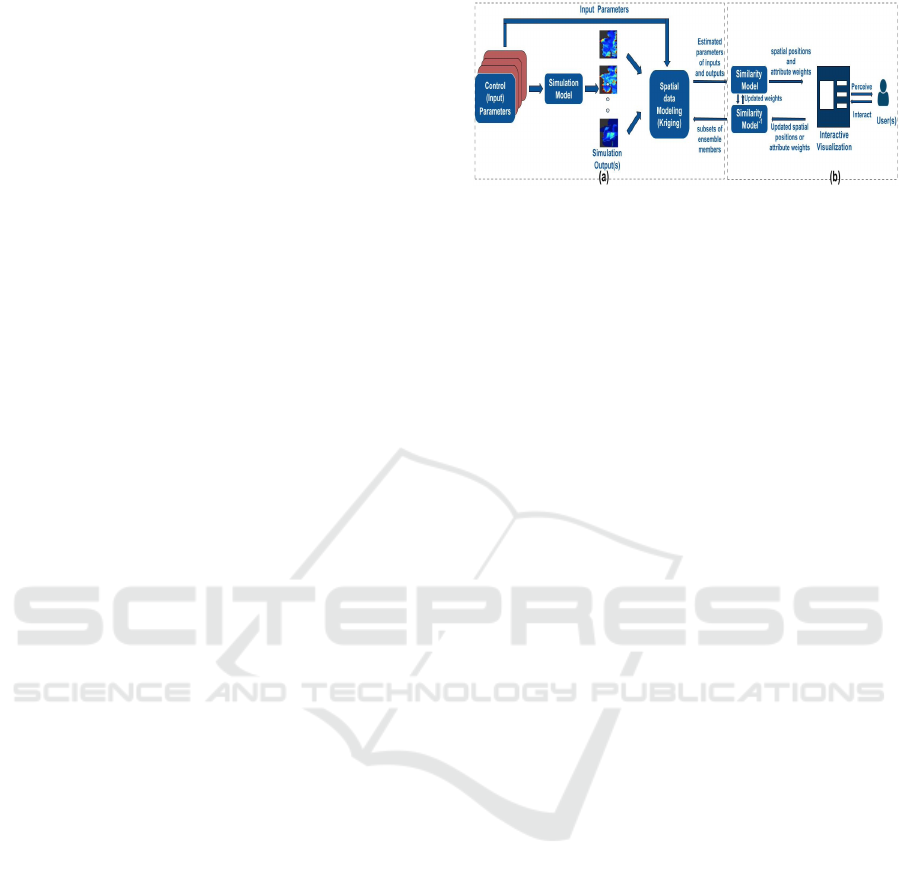
Figure 1: The workﬂow of our proposed visual analytical

approach. Our approach has two main steps: a) Statistical

modeling of the ensemble while considering spatial char-

acteristics in the data. b) Interactive visual exploration and

analysis of ensemble members, simulation parameters, and

spatial patterns.

models. Scientists aim to understand and analyze: 1)

ROI’s spatial characteristics within the ensemble to

ﬁnd features and patterns across members; 2) how

speciﬁc parameter or parameter settings affect ROI;

and 3) subsets of ensemble members to determine if

the relationship between input parameters holds for

the entire ensemble or only within speciﬁc subsets,

and vice versa.

Goal 4: Interactive Exploration and Comparison

of Spatial Distributions. Exploring the statistical at-

tributes of raw spatial data to uncover correlations and

static properties. This exploration involves analyzing

the data distribution to test hypotheses and verify ﬁnd-

ings.

3.2 System Overview

This section introduces our visual exploration frame-

work for the multidimensional spatial ensemble. The

proposed framework and its visualization components

align with the aforementioned tasks. Figure 1 pro-

vides a high-level overview of our approach. Our ap-

proach begins with an ensemble E of M members. In-

dividual ensemble members consist of input parame-

ters and simulation outputs (i.e., grid). Initially, we

model the simulation ensemble using GPR to esti-

mate spatial parameters that characterize each mem-

ber’s input parameters and simulation outputs. GPR

employs local MLE to determine various spatial pro-

cess features. These features are spatially smoothed

to capture the correlation structure between nearby

grid points. GPR does not require prior knowledge

of the ensemble member distribution. Thus, it can

uncover each ensemble member’s variability, main

trends, and autocorrelations. The estimated spatial

parameters are subsequently inputted into the visual-

ization pipeline of SpatialGLEE.

SpatialGLEE’s coordinated multi-views (Fig-

ure 2), coupled with their supported interaction tech-

IVAPP 2024 - 15th International Conference on Information Visualization Theory and Applications

680

niques, empower scientists to explore and analyze

multidimensional spatial ensembles. Ensemble view

(Figure 2a) visualizes ensemble members by project-

ing them from higher-dimensional space to lower-

dimensional space (i.e., 2D) via a projection tech-

nique (e.g., MDS, t-SNE, etc.), using estimated spa-

tial parameters for simulation outputs and input pa-

rameters and weights associated with them. The po-

sitioning of ensemble members in the ensemble view

reﬂects relative distances, where members with sim-

ilar estimated attributes are placed close together,

while those with dissimilar attributes are positioned

farther apart.

Scientists explore and compare ensemble mem-

bers and data spatially within the ensemble view us-

ing two main interactions: observation-level inter-

action (OLI), subsetting of ensemble members, and

ROI selection within ensemble members. OLI is an

interaction technique built on the SI principles (En-

dert et al., 2012). It allows scientists to directly ma-

nipulate ensemble members to investigate and un-

derstand their commonalities and differences. The

subsetting feature allows scientists to navigate sub-

sets of ensemble members for a more in-depth anal-

ysis. This capability enables scientists to seamlessly

switch between overview-ﬁrst and detailed-ﬁrst anal-

ysis modes. Moreover, scientists can utilize the ROI

selection feature to identify speciﬁc spatial regions of

interest within the data. This feature is valuable when

dealing with a large grid where not all regions are

equally signiﬁcant to the analysis. This allows a fo-

cused exploration of regions with similar patterns or

trends, enhancing the effectiveness of the analysis.

Parameter view (Figure 2b) offers scientists the

opportunity to investigate parameter sensitivity using

ensemble attributes (i.e., input parameters and out-

puts). Each attribute is represented on a horizontal

slider. The slider’s value represents the weight of

the attribute in the model, thereby marking its im-

portance. Using a Parametric Level Interaction (PLI),

scientists are able to manipulate the slider in order to

interact with model attributes. PLI allows scientists

to investigate associations and relationships between

input parameters and explore their impact on the sim-

ulation outputs.

Conversely, the statistical view (Figure 2c) helps

ﬁnd the optimal parameter settings. This view allows

scientists to explore raw data through various statisti-

cal representations, such as parallel coordinates, scat-

terplots, and boxplots. By leveraging these differ-

ent displays, scientists can determine variability in

the data, validate conclusions, identify hidden corre-

lations not found by other views, and gain insights

into the distribution of different ensemble members.

4 SPATIAL ENSEMBLE

MODELING

Simulation inputs and outputs serve as entry points

to SpatialGLEE’s visualization pipeline. Passing spa-

tial ensemble raw data directly to the visualization

pipeline would capture the spatiality in the data dur-

ing the exploration and analysis. However, it poses

computational challenges due to the complexity and

size of the ensemble. Therefore, there is a need for

modeling the spatial ensemble data while preserving

the underlying spatial structure.

Given a multidimensional spatial ensemble E=

,...K

} with M members, where each K

∈ E

is of a 2D grid G. Every grid point within K

is linked

to input and output values obtained from spatial simu-

lation assessments or measurements conducted across

the entire grid. K

represents a spatial stochastic pro-

cess {Q(s) : s ∈ G} with the spatial domain G ⊂ R

d≥1 (d vector of coordinates)(Dahshan, 2021). We

model Q(s) by

Q(s) = X (s)β+ w(s) + ε, (1)

so that Q(s) has mean X(s) β and error w(s) + ε. The

mean is the result of the product between the coef-

ﬁcients β and X(s), which represents a vector of p

co-variates at locations S. The additive error adds a

spatial-dependent error term, w(s), and an indepen-

dent measurement error term, ε, characterized by a

zero mean and variance τ

. The spatial dependence is

imposed by modeling w(s) as a stationary, mean-zero

spatial process with a covariance function

(s − s

′

) = σ

g(||Σ

−1/2

(s − s

′

)||), (2)

g() represents a spatial kernel covariance function that

operates on the distance between two grid points, and

serves as a covariance inﬂation term. Spatial co-

variance kernel functions establish the characteristics

and degree of spatial dependence within the spatial

process. For instance, they can establish greater de-

pendence between spatial outcomes when they are

close compared to those at a greater distance.

Based on the discussions with our collaborators,

we learned that their primary focus lies in understand-

ing spatial autocorrelation and variability in the en-

semble. According to Tobler’s 1st Law of Geography

(Miller, 2004), spatial autocorrelation expects nearby

spatial grid points to be more similar than far apart

ones. Therefore, our proposed approach ﬁts GPR

azaro-Gredilla et al., 2010), also known as Krig-

ing, to learn the characteristics of spatial processes.

Kriging provides a method for interpolating between

grid points. These interpolations maintain the spatial

correlation and variability present in the data.

Human-Machine Collaboration for the Visual Exploration and Analysis of High-Dimensional Spatial Simulation Ensembles

681

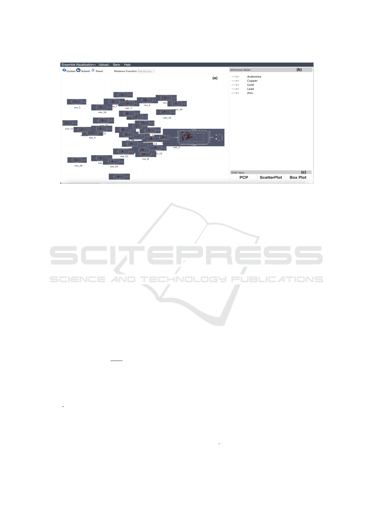
Figure 2: SpatialGLEE’s main interface:(a) Ensemble view shows the WMDS projection of the simulation ensemble in 2D

space. Ensemble members are spatially arranged so that similar ensemble members are near each other and dissimilar en-

semble members are far apart. Scientists can interactively manipulate image thumbnails representing ensemble members to

explore and analyze them. (b) Parameter view presents the weights assigned to both input parameters and simulation outputs.

Scientists can alter the slider values to examine the impact of the ensemble attributes. (c) Statistical view offers multiple

statistical displays to explore and understand the distributions, patterns, trends, and outliers in ensemble raw data.

With simulation measurements Y (s

) of N grid lo-

cations s

(i ∈ {1,...,N}). Estimating the process Y at

a new location s

, denoted Y

∗

) is a two-step pro-

cess. The process begins by ﬁtting a variogram to as-

certain the spatial covariance structure and parameters

based on observed data. Subsequently, it calculates

weights, denoted as λ

, from the covariances between

each observed location s

and the new location s

. The

value Y

∗

) is then derived from a weighted average.

∗

) =

∑

i=1

Y (s

). (3)

In our approach, we model a second-order station-

arity Gaussian Process (GP) with an isotropic Matern

covariance kernel. (Nychka et al., 2002). The Matern

covariance function is

C(d|κ,ν,σ

) = σ

ν−1

Γ(ν)

(d/κ)

(d/κ) (4)

where d is the Euclidean distance between s and s

′

(||s − s

′

||), Γ(.) is the gamma function, ν is a smooth-

ing parameter that controls the mean square differen-

tiability of the process (ν > 0), κ is a range parameter,

and K ν(.) is the modiﬁed Bessel function of second

kind order. We selected the Matern covariance be-

cause it offers signiﬁcant ﬂexibility in modeling spa-

tially correlated random processes. The smoothness

parameter associated with Matern covariance allows

control over the level of smoothness in the spatial pro-

cess.

To estimate model parameters, Kriging maximizes

the likelihood of the simulation measurements gen-

erating ﬁve estimates: nugget variance, scalar MLE

for kappa, anisotropy parameters (lam1, lam2), and

process variance. The computation of these estimates

relies heavily on matrix operations. The distance ma-

trices and covariance utilized in these operations cap-

ture the pairwise correlations among the locations of

the grid. As the spatial grid size increases, the com-

putational cost of kriging escalates, restricting its fea-

sibility with large datasets. To tackle this challenge,

various approaches have emerged, falling into two

categories: sparse approximations (Kaufman et al.,

2008) and local approximations (Wackernagel, 2013).

Sparse approximations involve approximating the co-

variance matrix with sparse matrices. Conversely, lo-

cal approximations partition input data into local and

independent regions, with each spatial region encom-

passing a relatively small number of local points clos-

est to the prediction point. Despite their ability to han-

dle large datasets, these approximation approaches

rely on some form of approximation, introducing the

risk of information loss and errors, thereby limiting

the advantages of using kriging.

Our aim is to implement a scalable high-

performance parallel and distributed version of the

MLE of the Kriging model. This implementation

leveraged multi-core and multi-node architectures to

boost computational performance. We leveraged

the Aniso ﬁt() API from the ConvoSPAT package of

R (Risser and Calder, 2015) for our implementation.

IVAPP 2024 - 15th International Conference on Information Visualization Theory and Applications

682

We modiﬁed the Aniso ﬁt() MLE implementation to

evaluate the maximization function and the function

returning the gradient for the same parameter value in

parallel. We used the Parallel package from R, which

supports multi-core and multi-node parallelization.

5 SPATIAL ENSEMBLE VISUAL

EXPLORATION

SpatialGLEE’s modeling and visualization aim to in-

vestigate similar behaviors and key parameters in the

ensemble, aligning with design goals. Scientists can

use SpatialGLEE’s multi-linked views and interac-

tion techniques to explore and analyze spatial ensem-

bles. SpatialGLEE integrates scientists’ intuition and

expertise with machine learning and statistics, facil-

itating the analysis and exploration of multidimen-

sional spatial ensembles. The visualization pipeline

of SpatialGLEE is comprised of three main compo-

nents: the input source, similarity models, and co-

ordinated visual interfaces. The spatially estimated

simulation outputs and input parameters serve as the

input source, processed through similarity models for

2D projection and manipulation. Coordinated multi-

views facilitate analysis, providing a comprehensive

understanding of spatial relationships and patterns in

the data.

5.1 Spatial Ensemble Attributes

The SpatialGLEE visualization pipeline employs the

spatial estimates (i.e., anisotropy parameters (lam1,

lam2), nugget variance, process variance, and scalar

MLE for kappa) as a foundation for spatial ensemble

analysis and exploration. To ensure an accurate unbi-

ased representation of the data during the exploration

and analysis of the spatial ensemble, these estimates

are z-score normalized. This normalization process

helps standardize the data and ensures that each es-

timate is considered in the context of its distribution,

preventing any skewed or misleading interpretations.

In addition, an initial weight of (1/ d) is assigned to

each attribute (i.e., inputs and outputs), where d is the

total number of simulation outputs and input parame-

ters. The weight of each attribute is evenly distributed

among its estimates, resulting in a weight of (1/5d)

for each individual estimate.

5.2 Similarity Models

The similarity models in SpatialGLEE manage the

visualization and interaction of simulation ensem-

ble data through two models: forward and back-

ward. The forward model utilizes weighted mul-

tidimensional scaling (WMDS) to project multidi-

mensional ensemble data into two-dimensional space.

This weighted projection integrates a weighted dis-

tance function to capture commonalities and distinc-

tions between ensemble members based on spatially

estimated attributes. The determination of the dis-

tance function in SpatialGLEE depends on the data

characteristics, the task, and the projection technique.

The primary interface offers scientists a range of dis-

tance functions to choose from, including weighted

Cosine, weighted Euclidean, and weighted Manhat-

tan, with the default being the weighted Mahalanobis

distance. The Mahalanobis distance measures the dis-

tance between any point in space and the distribu-

tion’s center, taking into account correlations between

attributes.

To explore ensemble members described by spa-

tial estimates of d parameters, WMDS is applied us-

ing weighted distance D

(i, j), for ensemble mem-

bers i and j ( i, j ∈ {1,...,M}), with weight w

rep-

resenting the weight applied to each spatial estimate

to denote its signiﬁcance in the projection. The pair-

wise distance function result between ensemble mem-

bers is subsequently inputted into WMDS. WMDS

determines the position of each individual member in

the low dimensions by minimizing the mean squared

error between the pairwise distances in two dimen-

sions and the corresponding distances in the high-

dimensional space.

The backward model is activated when scientists

interact with SpatialGLEE’s different views using dif-

ferent interaction techniques (i.e., OLI, PLI, brush-

ing, or subsetting). OLI enables scientists to create

a customized spatialization of multidimensional en-

semble members based on their intuition and domain

expertise. For instance, the expertise of the scien-

tists may contradict the spatialization of the ensem-

ble members, or they may observe interesting patterns

in the data. In response, they perform an OLI by

dragging subsets of ensemble members into groups.

These groupings signify scientists’ hypothesized sim-

ilarity between these ensemble members. The back-

ward model is then triggered, calling upon a semi-

supervised metric learning model. This model at-

tempts to learn new weights that correspond to the

identiﬁed similarity and subsequently adjusts the pro-

jection. Thus, OLI facilitates the exploration of re-

lationships and associations between ensemble mem-

bers by allowing scientists to shape the spatialization

based on their insights and hypotheses.

PLI empowers scientists to explore parameter sen-

sitivity by directly manipulating the attribute’s weight

Human-Machine Collaboration for the Visual Exploration and Analysis of High-Dimensional Spatial Simulation Ensembles

683

on the slider. This interaction results in an updated

weight vector and a new projection of ensemble mem-

bers based on the manipulated weight on the slider.

Given that all weights are constrained to add up to

one, increasing the weight of one attribute necessi-

tates decreasing the weights of all other attributes,

and vice versa. Thus, the updated projection ampli-

ﬁes the similarities and differences among data points,

intensifying with an increase in weight and diminish-

ing with a decrease in weight. This enables scientists

to offer parametric feedback to the backward model

regarding which attribute they consider to be signiﬁ-

cant and to observe how this attribute affects ensem-

ble members’ low-dimensional grouping. This inter-

action facilitates the exploration of the inﬂuence of

individual attributes on the spatial representation, al-

lowing scientists to gain insights into parameter sen-

sitivity within the ensemble.

The average size of a spatial simulation grid may

surpass millions of grid cells. In this case, scientists

might be interested in examining speciﬁc regions, like

those near wells or aquifers. The SpatialGLEE ROI

selection feature enables the interactive selection of

an ROI within the ensemble member within thumb-

nails in the ensemble view. Scientists can explore ROI

in two ways: either exclusively focusing on an ROI or

assigning a higher weight to it compared to other re-

gions on the grid. Exploring a speciﬁc ROI across all

ensemble members triggers the backward model, up-

dating the visualization pipeline with a newly updated

weight vector for spatial estimates of the chosen sub-

region of interest and thus adjusting the projection ac-

cordingly. On the other hand, increasing the weight of

a particular ROI triggers the backward model, which

updates the weight vector by dividing the weights be-

tween ensemble estimated attributes and subregion of

interest estimated attributes based on a percent deter-

mined by the scientist.

5.3 Coordinated Multi-View

Visualizations

SpatialGLEE’s multi-coordinated views, Figure 2,

contain an ensemble view, a parameter view, and a

statistical view.

Ensemble View: visualizes multidimensional ensem-

ble members in two-dimensional space using WMDS

to provide an overview of spatial ensemble data.

Each ensemble member is presented through a two-

dimensional image of the simulation output. The en-

semble view offers two main interactions: OLI and

ensemble members and ROI selection. These two in-

teractions provide scientists with an interactive explo-

ration environment for analyzing simulation ensem-

ble members, thereby contributing to achieving the

second and third design goals.

Parameter View: represents simulation input param-

eters and output parameters on horizontal sliders, with

each attribute represented by a single slider whose

value is the attribute’s weight. The weight of each

attribute is the sum of the weights of all its estimates.

Scientists utilize PLI within parameter view to inves-

tigate parameter sensitivity, achieving the ﬁrst design

goal.

Statistical View: supports other views by allowing

scientists to validate assumptions and reﬁne hypothe-

ses derived from other views. It offers three statisti-

cal displays—parallel coordinates, boxplot, and scat-

ter plot—supporting univariate, bivariate, and multi-

variate analyses. It can also be used to gain insights

into data distributions, identify the variability across

different regions, discover new patterns undiscovered,

or/and produce novel hypotheses that other views

could conﬁrm, thereby contributing to achieving the

fourth design goal. Statistical View offers statistical

displays for individual ensemble members, multiple

ensemble members, and speciﬁc regions within en-

semble members. For instance, scientists can explore

correlations between ensemble members or analyze

the distribution of single or multiple ensemble mem-

bers across the entire grid or speciﬁc subsets.

6 EVALUATION

We evaluated our proposed approach using a 2D spa-

tial ensemble from geologic CO2 sequestration. Dur-

ing the evaluation, we examined the effectiveness of

the proposed approach in aiding scientists to explore

and analyze multidimensional spatial ensembles. Our

emphasis was on gauging how well the approach fa-

cilitates the exploration of parameter sensitivity and

optimization, as well as the examination of similar-

ities and differences among ensemble members and

spatial regions of interest. Speciﬁcally, we investi-

gated the extent to which the statistically estimated

parameters could preserve the spatial structure during

exploration and analysis.

Three geoscience domain scientists (two gradu-

ate students and a faculty member) evaluated the pro-

posed approach. The faculty member supplied the en-

semble data used in the experiment. To initiate the

evaluation, the scientists received instructions on how

to use SpatialGLEE and its interaction techniques.

Subsequently, they were tasked with utilizing Spatial-

GLEE’s interaction techniques and visual interfaces

to explore and analyze the ensemble. Throughout the

evaluation, we recorded both the duration to complete

IVAPP 2024 - 15th International Conference on Information Visualization Theory and Applications

684

each task and the level of task completion. Addition-

ally, we timed every interaction that the domain ex-

perts carried out.

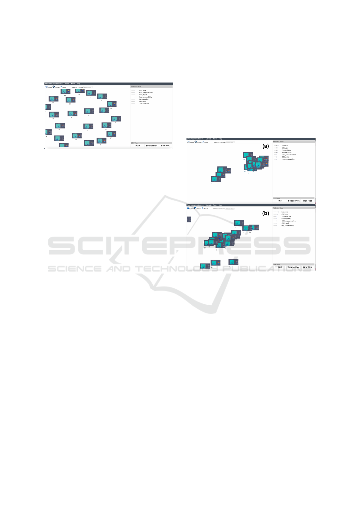
Figure 3: The initial projection of the multidimensional

CO2 ﬂow ensemble using spatially estimated simulation at-

tributes.

6.1 Case Study

The simulation ensemble study examines the multi-

phase ﬂuid dynamics of CO2 ﬂow in a basalt frac-

ture network (Gierzynski and Pollyea, 2017). The

model domain has a 2-D fracture network based on

high-resolution LiDAR scans of a basalt outcrop in

the Columbia River Plateau. The 5 m x 5 m model

domain is divided into 40,000 2.5 cm x 2.5 cm Carte-

sian grid cells. The study constructed a simulation

ensemble that randomly assigns fracture permeabil-

ity to each grid cell from a basalt core sample per-

meability distribution because centimeter-scale frac-

ture permeability is unknown. Thus, the ensemble has

25 equally probable model domains with permeabil-

ity spatial distribution as the random variable. Using

e-type estimations, this simulation ensemble exam-

ined how permeability impacts buoyant CO2’s ﬂow

characteristics during geologic CO2 sequestration in

a basalt reservoir as it phases from supercritical ﬂuid

to subcritical gas.

Figure 3 shows the initial projection of a multidi-

mensional CO2 ﬂow ensemble in 2D space. The sci-

entist didn’t observe any interesting patterns or groups

in the initial projection. The scientist was interested

in understanding the parametric controls of the phase

change to gas because the gas phase CO2 is sig-

niﬁcantly more buoyant and therefore has a greater

chance of leaking out of the CO2 storage reservoir.

To investigate this, the scientist started grouping en-

semble members into two groups based on how much

CO2 has moved to the upper portion of the model,

which is where the CO2 undergoes a phase change to

a gas phase, performing an OLI (Figure 4 a).

The reprojection of the ensemble revealed that

there was a notable increase in the weight of gas-

phase CO2, permeability, and ﬂuid pressure, as il-

lustrated in Figure 4b. This led the scientist to con-

clude that ﬂuid pressure is the dominant control for

this grouping. The rationale behind this conclusion

is that the phase change from supercritical CO2 to

gas-phase CO2 occurs as the CO2 ﬂoats to shallower

depths, where ﬂuid pressure is lower. Additionally,

the scientist gained insights from this reprojection that

permeability affects CO2 ﬂow; this necessitates addi-

tional experiments to determine how permeability dis-

tributions vary between ensemble members that ex-

hibit phase change and those that do not.

Figure 4: Investigating migration CO2 ﬂow using OLI: a)

semantically grouping ensemble members from the CO2

ﬂow ensemble into two clusters based on how much CO2

has moved to the upper portion of the model; b) The re-

sulted projection shows permeability and ﬂuid pressure (P)

have a dominant role in the phase change from supercritical

CO2 to gas-phase CO2.

The scientist wanted to investigate the effect of

ﬂuid pressure alone on the ensemble, so s/he con-

ducted PLI by increasing the ﬂuid pressure’s weight.

However, the reprojection result was inconclusive.

So, the scientist decided to explore if the tempera-

ture has any inﬂuence on the ensemble by perform-

ing PLI (Figure 5). The resulted projection was a

linear projection in which ensemble members with

high CO2 gas at shallow depths close to the top of

the workspace. This discovery led the scientist to ob-

serve that there is a thermal control on the CO2 phase

change, but it is much more subtle in the ensemble.

This was a new discovery that required a more de-

tailed analysis.

The scientist was interested in determining

whether log permeability affects the ensemble. So,

Human-Machine Collaboration for the Visual Exploration and Analysis of High-Dimensional Spatial Simulation Ensembles

685

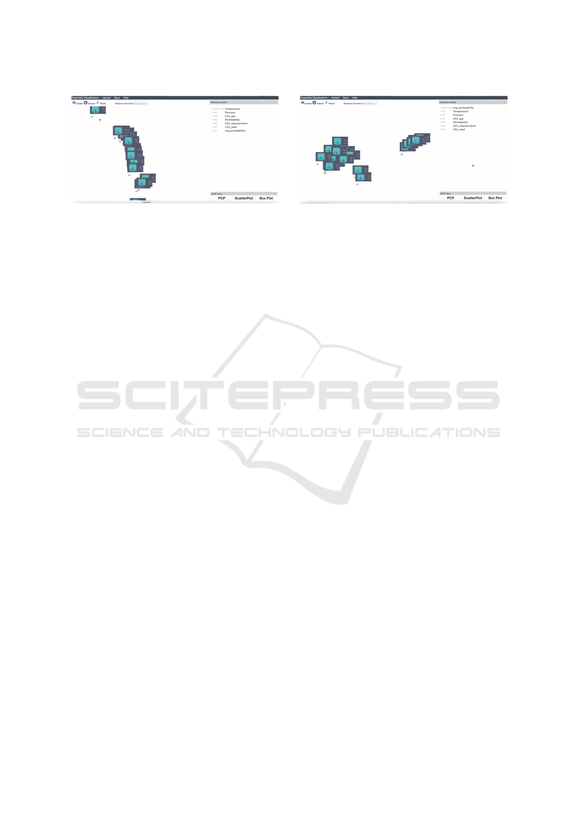
Figure 5: Increasing the weight of the temperature attribute

while performing PLI to explore its impact on the ensemble.

The resulted projection led to the conclusion that there is a

thermal control on the CO2 phase change.

s/he increased the weight of log permeability per-

forming an PLI (Figure 6). The projection resulted

in the separation of ensemble members into distinct

piles. The pile on the right has low CO2 gas at shal-

low depths, whereas the pile on the left has high CO2

gas concentrations at shallow depths. This led the sci-

entist to conclude that the pile on the right has low

permeability in the conductive fracture shallow depth,

which keeps ﬂuid pressure high and prevents the CO2

from undergoing phase change to CO2 gas.

After interacting with SpatialGLEE through var-

ious interactions, the scientist aimed to identify po-

tential patterns among parameters and investigate

whether the distribution of raw data for different pa-

rameters varied across runs. To explore this, the sci-

entist employed statistical view displays (Figure 7).

The use of a boxplot showed that the distribution of

log permeability remained consistent across all runs.

Furthermore, a scatter plot uncovered a moderately

positive correlation between pressure and CO2 se-

questration, as well as a positive correlation between

CO2 sequestration and CO2 total. By employing par-

allel coordinates, the scientist detected a correlation

among log permeability, temperature, and CO2 gas

across speciﬁc runs.

The scientist aimed to investigate regions of inter-

est (ROI) within the reservoir. To facilitate this ex-

ploration, s/he resets the ensemble view to obtain a

new projection. Subsequently, s/he selected a partic-

ular run and identiﬁed a ROI. SpatialGLEE supports

two exploration options for ROI: either allocate a per-

centage of the weight vector to this ROI and explore

it concurrently with the entire reservoir or assign the

entire weight vector exclusively to this speciﬁc ROI.

The scientist explored both options while using Spa-

tialGLEE interaction techniques and determined that

speciﬁc characteristics in these ROIs required further

investigation through higher-ﬁdelity simulations (Fig-

ure 8.

Figure 6: Performing a PLI to investigate the effect of in-

creasing the log permeability weight on the ensemble. The

resulted projection led to the conclusion that low permeabil-

ity in the conductive fracture shallow depth keeps ﬂuid pres-

sure high and prevents CO2 from undergoing phase change

to CO2 gas.

6.2 Domain Expert Evaluation

We discussed the SpatialGLEE tool and its interac-

tion techniques with the domain experts who pro-

vided the ensemble data for the case study. We so-

licited their feedback on the usability and utility of

SpatialGLEE. Scientists conﬁrmed that by using Spa-

tialGLEE, they were able to reach conclusions in sig-

niﬁcantly less time compared to the traditional anal-

ysis process. SpatialGLEE coordinated views allow

them to simultaneously visualize, explore, and under-

stand parameter and ensemble spaces in the absence

of prior knowledge. The ensemble view allows an-

alyzing both ensemble members and spatial regions

within members. This helps them identify signiﬁ-

cant regions in the grid. The parameter view permits

them to directly investigate input parameters’ effects

on simulation outputs. The statistical view supports

scientists in locating interesting patterns in raw spatial

data and exploring them using SpatialGLEE’s views

and interaction techniques. It also helps in ﬁnding the

optimal parameter settings. SpatialGLEE has the po-

tential to aid in the discovery of new insights that ne-

cessitate additional experiments for in-depth analysis.

6.3 Discussion

SpatialGLEE Showed the Potential to Improve

Spatial Ensemble Exploration over Traditional

Approaches. SpatialGLEE presents an approach for

exploring multidimensional spatial ensembles when

scientists do not have an in-depth understanding of the

simulated model. Traditionally, scientists utilize visu-

alizations of simulation outputs and summary statis-

tics to investigate the variability of an individual pa-

rameter (whether input or output) throughout the en-

tire ensemble. This traditional approach often ne-

IVAPP 2024 - 15th International Conference on Information Visualization Theory and Applications

686

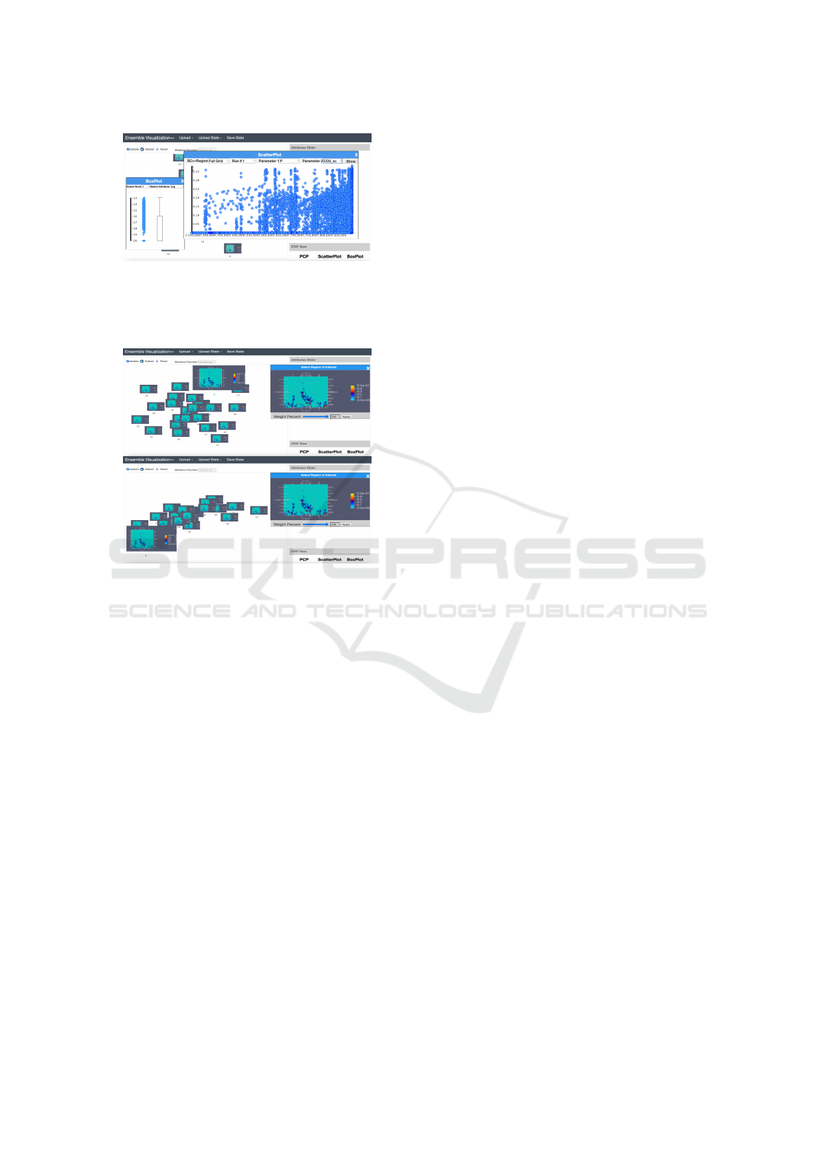
Figure 7: Exploring the distributions and correlations be-

tween parameters of raw spatial data utilizing the statistical

view. This view shows statistical distributions and proper-

ties of data using univariate, bivariate, and multivariate sta-

tistical displays.

Figure 8: Spatial Region of Interest (ROI) Selection: a) The

scientist was interested in exploring a certain region within

the reservoir, so s/he selected the ROI and increased its im-

portance over other regions in the grid by 100%. b) The

ensemble members are re-projected based on the newly up-

dated weight vector.

cessitates the implementation of several programs or

scripts for data visualization, which takes a substan-

tial amount of time and increases the risk of errors.

In our comparison between the insights and conclu-

sions generated by SpatialGLEE and those obtained

through the scientist’s regular analysis process, we

found that SpatialGLEE led to the same conclusions

as the manual analysis process but in signiﬁcantly less

time. Furthermore, SpatialGLEE facilitated the dis-

covery of new phenomena and insights that would be

challenging to uncover using traditional methods.

The qualitative analysis of the study reveals that

using OLI, the scientist was able to ﬁgure out com-

monalities and differences across ensemble members

and within ROI in ensemble members based on

speciﬁc patterns or hypotheses. The resulted projec-

tion from OLI provides scientists with the ability to

identify which parameter(s) guide the grouping of

ensemble members. However, OLI is a technique

for exploratory interaction; therefore, it would not

always generate signiﬁcant outcomes. Obtaining

signiﬁcant insights or even discoveries would be

possible if the grouped ensemble members shared

high-dimensional features that could be captured

by the metric learning model. Utilizing the PLI,

scientists managed to identify the sensitivity of input

parameters to the simulation output. This facilitated

the identiﬁcation of crucial parameters and those

that could be set as constants in the simulation. On

the other hand, through the use of statistical view

displays, scientists were able to explore and analyze

raw data from spatial ensembles. This helped them

understand the distribution and variability of the data,

leading to the identiﬁcation of optimal parameter

settings for the input parameters.

SpatialGLEE Performance. Our quantitative mea-

surements demonstrate that the interaction techniques

of SpatialGLEE allow scientists to accomplish all

preliminary exploration tasks. However, when

interacting with SpatialGLEE, additional exploratory

inquiries emerged. The scientists addressed some

of these inquiries, but others demanded simulations

of greater ﬁdelity. We computed the total number

of interactions needed to answer the preliminary

exploration tasks. This count varied among scien-

tists, depending on the nature of the interactions

they performed within the ensemble. For example,

completing the preliminary exploration tasks needed

on average took 1–5 interactions. Advanced tasks

that emerged during the analysis exhibit variability in

the number of interactions, ranging from an average

of 3 to 8. Additionally, SpatialGLEE responded

to the interactions of scientists within a reasonable

time frame. Responding to OLI, PLI, and ensemble

member and ROI selection required less than 5s, 3s,

and 1s respectively.

Spatial Ensemble Modeling. Modeling spatial en-

sembles using GPR preserves the spatiality of the

data during exploration and analysis of both ensme-

ble members and ROI within the ensemble. Us-

ing the modeled data with SpatialGLEE interaction

techniques revealed that grouping ensemble members

captured the intrinsic structures and spatial charac-

teristics of the data. This provided scientists with

additional insights that might be challenging to ob-

tain using traditional visualization methods reliant

on summary statistics (i.e., standard deviation and

mean). Moreover, the parallel implementation of

MLE demonstrates superior computational perfor-

mance compared to conventional MLE. Our approach

is scalable, functioning effectively across both the

same node and multiple nodes (Figure 9). We con-

ducted our scaling evaluation on an Intel SkyLake

Xeon Gold cluster with 24 cores and 384 GB of mem-

Human-Machine Collaboration for the Visual Exploration and Analysis of High-Dimensional Spatial Simulation Ensembles

687

ory per node. We observed that while our implemen-

tation scales on multiple cores of the same node, using

multiple nodes leverages the aggregate cluster mem-

ory, resulting in further performance improvement.

On 8 nodes and 128 cores, our parallel implementa-

tion achieved approximately 8× speedup compared to

2 nodes and 16 cores. The total speedup compared to

the sequential Aniso ﬁt() implementation is 21×.

Figure 9: Execution time of parallel MLE on various cores

(i.e., 16, 32, 64, 128) across distributed nodes (i.e.,2, 4, 8)

Distance Function Learning Model. SpatialGLEE

is designed to assist scientists in exploring spatial

simulation ensembles. The projection of ensemble

members from high-dimensional space to 2D space

and their grouping in the ensemble view signiﬁcantly

inﬂuence the exploration process. In the forward

similarity SI model, the distance function can be

described as an interactive distance function learning

model. The selection of the distance function plays a

pivotal role in the forward similarity SI model and,

consequently, impacts the projection of ensemble

members. The interactive nature of the distance

function suggests that it may learn from the speciﬁc

characteristics of the data, contributing to a more

dynamic approach to determining similarities be-

tween the ensemble members. While the choice of

distance function is based on the characteristics of

the data and the task at hand, we observed different

performances of different distance functions (i.e.,

Euclidean, Manhattan, and Mahalanobis) when

using spatial ensembles. The Euclidean distance

only captures the general spatial arrangement in the

ensemble, providing limited insights to scientists.

Conversely, manhattan distance outperforms eu-

clidean distance due to its sensitivity to multivariate

outliers. In contrast, when compared to other distance

functions, Mahalanobis distance demonstrates greater

accuracy in grouping ensemble members. This can

be attributed to its consideration of the multivariate

covariance structure during distance calculation.

However, Mahalanobis distance comes with a notable

drawback: its computational complexity is high for

large datasets.

Limitations and Future Work. Increasing the num-

ber of ensemble members to the hundreds may result

in visual cluttering within the ensemble view. One po-

tential solution to the problem is using larger displays

that are capable of accommodating a greater number

of ensemble members. Based on scientists’ feedback,

it was observed that scientists typically opt for an en-

semble size that is smaller than one hundred. Our cur-

rent approach and its parallel implementation are tai-

lored for 2D spatial grids and do not currently provide

support for 3D grids. In our future work, we plan to

expand SpatialGLEE to add support for 3D grids and

incorporate the capability for handling time-varying

simulation ensembles.

7 CONCLUSION

In this paper, we proposed SpatialGLEE, a visual ex-

ploration approach for multi-dimensional spatial en-

sembles. The proposed approach modeled the spa-

tiality of data in ensemble members using Gaussian

Process Regression (GPR) and explored its feasibil-

ity for visual exploration with Semantic Interaction.

SpatialGLEE interactive visual interfaces and interac-

tions enabled scientists to explore commonalities and

distinctions across ensemble members, subsets of the

ensemble, and ROI within the ensemble. Addition-

ally, they were able to determine parameter sensitivity

and optimization, as well as analyze the statical prop-

erties of the raw spatial data of ensemble members

and their parameters. The effectiveness of our pro-

posed approach was evaluated through experiments

involving domain experts. We found that by employ-

ing the SpatialGLEE approach, scientists could effec-

tively explore spatial simulation parameter and en-

semble spaces simultaneously, potentially leading to

the generation of new ﬁndings and discoveries.

REFERENCES

Ahmed, K., Sachindra, D. A., Shahid, S., Demirel, M. C.,

and Chung, E.-S. (2019). Selection of multi-model

ensemble of general circulation models for the simula-

tion of precipitation and maximum and minimum tem-

perature based on spatial assessment metrics. Hydrol-

ogy and Earth System Sciences, 23(11):4803–4824.

Athawale, T., Maljovec, D., Yan, L., Johnson, C., Pascucci,

V., and Wang, B. (2020). Uncertainty visualization

of 2d morse complex ensembles using statistical sum-

mary maps. IEEE Transactions on Visualization and

Computer Graphics.

Cappello, F., Constantinescu, E., Hovland, P., Peterka, T.,

Phillips, C., Snir, M., and Wild, S. (2015). Improv-

ing the trust in results of numerical simulations and

scientiﬁc data analytics. Technical report, Argonne

National Lab.(ANL), Argonne, IL (United States).

IVAPP 2024 - 15th International Conference on Information Visualization Theory and Applications

688

Chen, X., Shen, L., Sha, Z., Liu, R., Chen, S., Ji, G., and

Tan, C. (2019). A survey of multi-space techniques in

spatio-temporal simulation data visualization. Visual

Informatics, 3(3):129–139.

Dahshan, M., Polys, N. F., Jayne, R., and Pollyea, R. M.

(2020). Making sense of scientiﬁc simulation ensem-

bles with semantic interaction. In Computer Graphics

Forum, volume 39, pages 325–343. Wiley Online Li-

brary.

Dahshan, M. M. S. I. (2021). Visual analytics for high di-

mensional simulation ensembles.

Demir, I., Dick, C., and Westermann, R. (2014). Multi-

charts for comparative 3d ensemble visualization.

IEEE Transactions on Visualization and Computer

Graphics, 20(12):2694–2703.

Endert, A., Fiaux, P., and North, C. (2012). Semantic inter-

action for sensemaking: inferring analytical reasoning

for model steering. IEEE Transactions on Visualiza-

tion and Computer Graphics, 18(12):2879–2888.

Evers, M. and Linsen, L. (2022). Multi-dimensional

parameter-space partitioning of spatio-temporal sim-

ulation ensembles. Computers & Graphics, 104:140–

151.

Favelier, G., Faraj, N., Summa, B., and Tierny, J. (2018).

Persistence atlas for critical point variability in en-

sembles. IEEE transactions on visualization and com-

puter graphics, 25(1):1152–1162.

Fofonov, A. and Linsen, L. (2018). Multivisa: Visual anal-

ysis of multi-run physical simulation data using inter-

active aggregated plots. In VISIGRAPP (3: IVAPP),

pages 62–73.

Fofonov, A. and Linsen, L. (2019). Projected ﬁeld similar-

ity for comparative visualization of multi-run multi-

ﬁeld time-varying spatial data. In Computer Graphics

Forum, volume 38, pages 286–299. Wiley Online Li-

brary.

Gierzynski, A. O. and Pollyea, R. M. (2017). Three-phase

co2 ﬂow in a basalt fracture network. Water Resources

Research, 53(11):8980–8998.

Huang, Q., Chen, Q., Liu, G., and Cui, Z. (2023). Visual-

ization facilitates uncertainty evaluation of multiple-

point geostatistical stochastic simulation. Visual In-

telligence, 1(1):12.

Huesmann, K. and Linsen, L. (2022). Similaritynet: A deep

neural network for similarity analysis within spatio-

temporal ensembles. In Computer Graphics Forum,

volume 41, pages 379–389. Wiley Online Library.

Kaufman, C. G., Schervish, M. J., and Nychka, D. W.

(2008). Covariance tapering for likelihood-based esti-

mation in large spatial data sets. Journal of the Amer-

ican Statistical Association, 103(484):1545–1555.

Kumpf, A., Stumpfegger, J., Hartl, P. F., and Westermann,

R. (2021). Visual analysis of multi-parameter distri-

butions across ensembles of 3d ﬁelds. IEEE Transac-

tions on Visualization and Computer Graphics.

azaro-Gredilla, M., Quinonero-Candela, J., Rasmussen,

C. E., and Figueiras-Vidal, A. R. (2010). Sparse spec-

trum gaussian process regression. The Journal of Ma-

chine Learning Research, 11:1865–1881.

Li, W., Duan, Q., Miao, C., Ye, A., Gong, W., and Di, Z.

(2017). A review on statistical postprocessing meth-

ods for hydrometeorological ensemble forecasting.

Wiley Interdisciplinary Reviews: Water, 4(6):e1246.

Liu, L., Padilla, L., Creem-Regehr, S. H., and House, D. H.

(2018). Visualizing uncertain tropical cyclone predic-

tions using representative samples from ensembles of

forecast tracks. IEEE transactions on visualization

and computer graphics, 25(1):882–891.

Miller, H. J. (2004). Tobler’s ﬁrst law and spatial analysis.

Annals of the Association of American Geographers,

94(2):284–289.

Mirzargar, M., Whitaker, R. T., and Kirby, R. M. (2014).

Curve boxplot: Generalization of boxplot for ensem-

bles of curves. IEEE transactions on visualization and

computer graphics, 20(12):2654–2663.

Nychka, D., Wikle, C., and Royle, J. A. (2002). Multires-

olution models for nonstationary spatial covariance

functions. Statistical Modelling, 2(4):315–331.

Orban, D., Keefe, D. F., Biswas, A., Ahrens, J., and Rogers,

D. (2018). Drag and track: A direct manipulation in-

terface for contextualizing data instances within a con-

tinuous parameter space. IEEE transactions on visu-

alization and computer graphics, 25(1):256–266.

Potter, K., Wilson, A., Bremer, P.-T., Williams, D., Dou-

triaux, C., Pascucci, V., and Johnson, C. R. (2009).

Ensemble-vis: A framework for the statistical visual-

ization of ensemble data. In 2009 IEEE International

Conference on Data Mining Workshops, pages 233–

240. IEEE.

Risser, M. D. and Calder, C. A. (2015). Local likelihood

estimation for covariance functions with spatially-

varying parameters: the convospat package for r.

arXiv preprint arXiv:1507.08613.

Shi, N., Xu, J., Li, H., Guo, H., Woodring, J., and Shen, H.-

W. (2022). Vdl-surrogate: A view-dependent latent-

based model for parameter space exploration of en-

semble simulations. IEEE Transactions on Visualiza-

tion and Computer Graphics, 29(1):820–830.

Shu, Q., Guo, H., Liang, J., Che, L., Liu, J., and Yuan, X.

(2016). Ensemblegraph: Interactive visual analysis of

spatiotemporal behaviors in ensemble simulation data.

In 2016 IEEE Paciﬁc Visualization Symposium (Paci-

ﬁcVis), pages 56–63. IEEE.

Vietinghoff, D., Bottinqer, M., Scheuermann, G., and

Heine, C. (2022). Visualizing conﬁdence intervals

for critical point probabilities in 2d scalar ﬁeld ensem-

bles. In 2022 IEEE Visualization and Visual Analytics

(VIS), pages 145–149. IEEE.

Wackernagel, H. (2013). Multivariate geostatistics: an

introduction with applications. Springer Science &

Business Media.

Wang, J., Hazarika, S., Li, C., and Shen, H.-W. (2018). Vi-

sualization and visual analysis of ensemble data: A

survey. IEEE transactions on visualization and com-

puter graphics, 25(9):2853–2872.

Wang, J., Liu, X., Shen, H.-W., and Lin, G. (2016). Multi-

resolution climate ensemble parameter analysis with

nested parallel coordinates plots. IEEE transactions

on visualization and computer graphics, 23(1):81–90.

Winsberg, E. (2013). Computer simulations in science.

Zhang, M., Chen, L., Li, Q., Yuan, X., and Yong, J. (2020).

Uncertainty-oriented ensemble data visualization and

exploration using variable spatial spreading. IEEE

Transactions on Visualization and Computer Graph-

ics, 27(2):1808–1818.

Human-Machine Collaboration for the Visual Exploration and Analysis of High-Dimensional Spatial Simulation Ensembles

689