Avoiding Undesirable Solutions of Deep Blind Image Deconvolution
Antonie Bro
ˇ
zov
´
a
1,2
and V
´
aclav
ˇ
Sm
´
ıdl
2
1
Faculty of Nuclear Sciences and Physical Engineering, Czech Technical University in Prague, Czech Republic
2
Institute of Information Theory and Automation, Czech Academy of Sciences, Czech Republic
fi
Keywords:
Blind Image Deconvolution, Deep Image Prior, No-Blur, Variational Bayes.
Abstract:
Blind image deconvolution (BID) is a severely ill-posed optimization problem requiring additional informa-
tion, typically in the form of regularization. Deep image prior (DIP) promises to model a naturally looking
image due to a well-chosen structure of a neural network. The use of DIP in BID results in a significant perfor-
mance improvement in terms of average PSNR. In this contribution, we offer qualitative analysis of selected
DIP-based methods w.r.t. two types of undesired solutions: blurred image (no-blur) and a visually corrupted
image (solution with artifacts). We perform a sensitivity study showing which aspects of the DIP-based algo-
rithms help to avoid which undesired mode. We confirm that the no-blur can be avoided using either sharp
image prior or tuning of the hyperparameters of the optimizer. The artifact solution is a harder problem since
variations that suppress the artifacts often suppress good solutions as well. Switching to the structural similar-
ity index measure from L
2
norm in loss was found to be the most successful approach to mitigate the artifacts.
1 INTRODUCTION
Recovery of a sharp, clean image from a degraded one
is a difficult task regardless of the type of degradation.
This paper is concerned with blur degradation, which
may be caused by the relative motion of a camera and
a scene, turbulence in the atmosphere, or the focus
of a camera. Assuming a spatially invariant blur, a
blurred image d can be represented as a convolution
(denoted by ⊛) of a point spread function (PSF) k and
an underlying sharp image x
d = k ⊛ x + n, (1)
where n denotes a noise matrix. The deconvolution
is basically an inverse operation to the convolution
with the aim of recovering the sharp image from the
blurred one. The deconvolution is called blind (BID)
when not only the sharp image but also the PSF is
unknown. The task is then to minimize
∥d − k ⊛ x∥, (2)
with respect to both x and k. To preserve the energy
of the image, k is required to contain only nonnegative
values and sum to 1.
Minimizing (2) is difficult since there can be many
local minima other than the ground-truth solution.
One notable solution is the trivial no-blur solution
reconstructing the observation by the blurred image
and Dirac delta PSF. Therefore, it is necessary to add
some regularizer to (2) or prior information that helps
recover the real sharp image x.
Sharp image priors were designed to yield a higher
probability of sharp images over blurred ones to steer
the optimization algorithm from the no-blur solutions,
starting with (Miskin and MacKay, 2000), (Likas and
Galatsanos, 2004) and (Molina et al., 2006). Vari-
ational Bayes (Tzikas et al., 2009), (Kotera et al.,
2017) and Maximum Aposteriori (MAP) (Levin et al.,
2011), (Perrone and Favaro, 2016) approaches were
mainly discussed and various priors were proposed
(Wipf and Zhang, 2014). Total variation (TV) min-
imizing the L1 norm of horizontal and vertical dif-
ferences of the sharp image was proposed among
first image priors (Chan and Wong, 1998). Later,
the strength of super-gaussian priors (Babacan et al.,
2009) was discovered. Similarly to TV, they assume
that the gradient of the sharp image is sparse and most
of its values is centered around zero. The priors do not
necessarily need to prefer the sharp image but rather
help to avoid the blurred one. Although these tradi-
tional methods are quite successful, their efficiency
depends on a blur type, and inverse operations often
leave the estimates of the sharp images degraded by
artifacts (see the left image in Figure 1).
A completely different approach to blind image
deconvolution is based on deep learning (Huang et al.,
Brožová, A. and Šmídl, V.
Avoiding Undesirable Solutions of Deep Blind Image Deconvolution.
DOI: 10.5220/0012397600003660
Paper published under CC license (CC BY-NC-ND 4.0)
In Proceedings of the 19th International Joint Conference on Computer Vision, Imaging and Computer Graphics Theory and Applications (VISIGRAPP 2024) - Volume 3: VISAPP, pages
559-566
ISBN: 978-989-758-679-8; ISSN: 2184-4321
Proceedings Copyright © 2024 by SCITEPRESS – Science and Technology Publications, Lda.
559

2023), (Zhao et al., 2022), (Asim et al., 2020). Su-
pervised deep learning models usually require train-
ing on large datasets, giving them more information
than the traditional methods get and, therefore, out-
performing them. However, there are real-world sce-
narios where large datasets are not available and for a
long time, the Bayesian methods have been state-of-
the-art for these problems. In 2018 (Ulyanov et al.,
2018) proposed Deep Image Prior (DIP), stating that
the structure of a deep neural network is a regular-
izer of the problem itself. It was shown that such a
neural network learns naturally smooth images faster
than noise, which, according to (Shi et al., 2022), is
caused by faster learning of low-frequency informa-
tion. They successfully used it for image denoising,
inpainting, and superresolution. (Ren and et al., 2020)
combined the DIP image network with a feedforward
neural network (FNN) representing the PSF in 2020
and proposed SelfDeblur. This model deblurs im-
ages without any training dataset and outperforms the
Bayesian methods. They also propose to use TV reg-
ularization, but unless the images are noisy enough, it
has no visible benefit. (Kotera et al., 2021) suggests
that its success is not caused only by the DIP, but by
some interplay between the structure of the network
and the optimizer.
DualDeblur (Shin et al., 2021) utilizes DIP and
multiple blurry images. (Wang et al., 2019) focus
on the PSF and represent it with DIP as well as the
sharp image. (Bredell et al., 2023) combined the DIP
with Wiener deconvolution. The two conceptions of
the ‘prior’ have been combined by (Huo et al., 2023),
where the DIP-based model was complemented by
the sharp image prior and BID solved as minimiza-
tion of the variational lower bound.
However, all presented methods report only the
average PSNR of the restored images without a de-
tailed analysis of the effect of the components of their
method. In this contribution, we analyze the effect
of selected variations of DIP deblurring to shed some
light on their role in the quality of the restoration.
Specifically:
1. We demonstrate that DIP-based deconvolution is
an intrinsically stochastic process, and thus it can
be understood only via statistical methods analyz-
ing full distribution.
2. We focus on two specific types of undesired solu-
tions, the ”no-blur” and ”artifact” solutions, and
propose a PSNR-NB metric to distinguish them.
3. We demonstrate experimentally that the no-blur
solution can be avoided by choosing the optimiza-
tion hyperparameters well or by the sharp image
priors.
4. We illustrate that the suppression of the artifact
solutions is a much more demanding task and is
greatly influenced by the stochasticity of the DIP-
based methods. The most significant improve-
ment seems to be brought by switch to SSIM loss
during optimization.
2 BACKGROUND AND
MOTIVATION
Here, we will shortly review the analyzed methods,
demonstrate their stochastic nature, and formulate the
research objectives.
2.1 Deep BID Methods
We now introduce the studied algorithms SelfDeblur
and VDIP, and a simplification of the SelfDeblur al-
gorithm that reveals some properties of the MAP ap-
proach.
SelfDeblur. (Ren and et al., 2020) combines two
generative neural networks: G
x
representing x and G
k
representing k. The estimates of x and k are generated
by inputting fixed random arrays z
x
and z
k
, into the
networks. G
x
is a 5-level U-net (Ronneberger et al.,
2015) with skip connections and bilinear upsampling.
G
k
is a FNN with one hidden layer. Softmax at the
output of G
k
preserves the L
1
norm of the PSF. The
minimized loss is
L
SDB
(θ
k
, θ
x
) = MSE (d, G
k
(θ
k
|z
k
) ⊛ G
x
(θ
x
|z
x
)),
(3)
where θ
x
, resp. θ
k
represents the trainable parame-
ters of G
x
, resp. G
k
. The two networks are opti-
mized jointly in 5000 epochs using Adam optimizer
(Kingma and Ba, 2014) with learning rates (LR)
η
x
= 10
−2
for G
x
and η
k
= 10
−4
for G
k
. LRs are
halved in 2000
th
, 3000
th
and 4000
th
iterations and z
x
is perturbed by Gaussian noise with the standard de-
viation of 0.001 in every iteration. Although not in
the original paper, the code provided by authors con-
tains a switch to SSIM loss (5) after 1000 iterations.
(Kotera et al., 2021) reported that this switch some-
times causes the optimization to deteriorate, so it will
not be used as default in this method.
SimplerSDB. A slightly simpler model is also used
in this paper. x is represented by G
x
from SelfDeblur,
but k is represented only by an array θ
k
normalized
by softmax function (denoted as σ(.)). The deconvo-
lution is then formulated as the minimization of
L
SSDB
(θ
k
, θ
x
) = MSE (d, σ(θ
k
) ⊛ G
x
(θ
x
|z
x
)). (4)
VISAPP 2024 - 19th International Conference on Computer Vision Theory and Applications
560

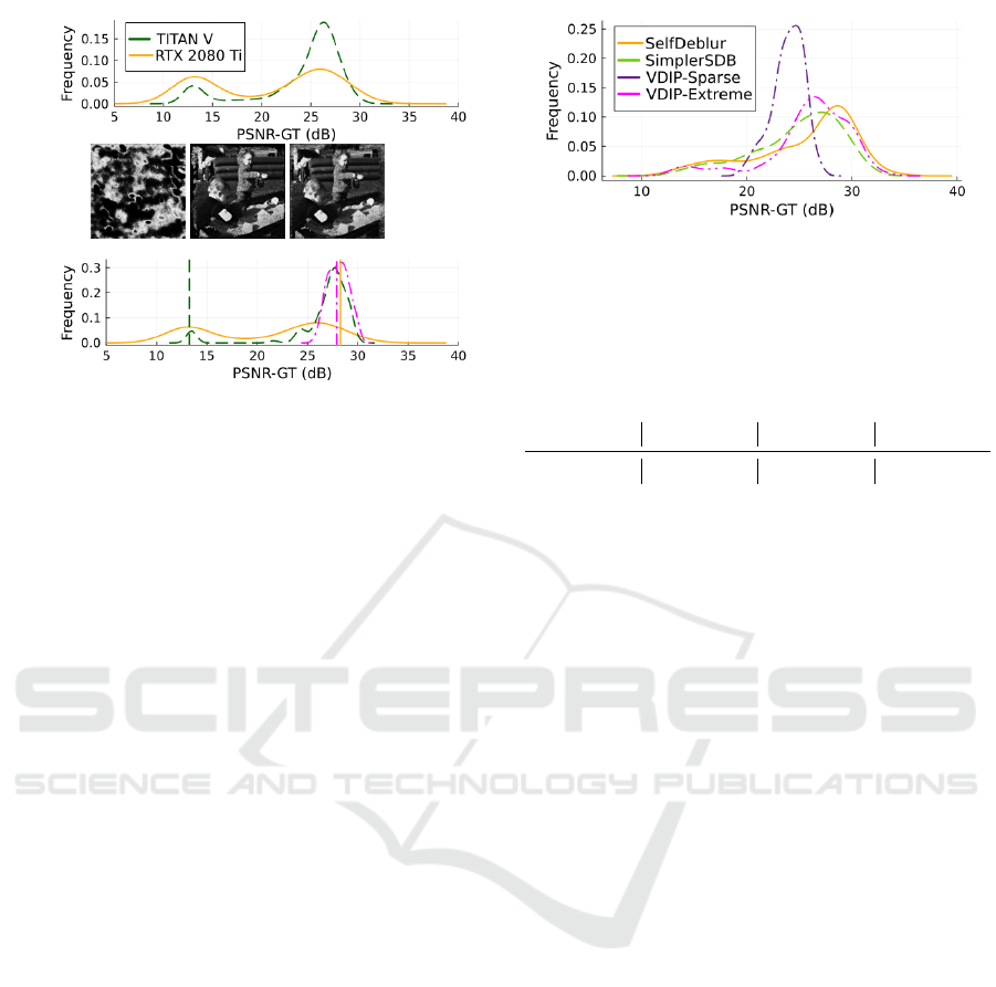
(a)
(b)
Figure 1: Illustration of stochastic influences. (a) PSNR
histograms of nondeterministic computations on two GPUs.
(b) PSNR histograms for three different initial values and
nondeterministic computations on NVIDIA GeForce RTX
2080 Ti. The vertical lines show the PSNR of a result ob-
tained by deterministic operations from corresponding ini-
tial values. The three reconstructed images are displayed
above the graph.
The parameters are again optimized by Adam op-
timizer and η
k
= η
x
= 10
−2
. Random perturbations
of z
x
and learning rate scheduling used in SelfDeblur
are turned off. This algorithm, stripped of everything
else but DIP, will be called SimplerSDB.
Variational BID: VDIP. The last algorithm used in
this paper for comparison is VDIP (Huo et al., 2023)
utilizing two priors for the sharp image: sparse one
(VDIP-Sparse) and extreme channel prior (Yan et al.,
2017) (VDIP-Extreme). G
x
and G
k
are the same as in
SelfDeblur. VDIP not only utilizes the DIP but also
adds stronger prior information similar to bayesian
methods. Apart from that, the considered loss is
MSE-like (3) only in the first 2000 iterations; for the
next 3000, it is switched to SSIM (structural similar-
ity index measure) (Wang et al., 2004) loss, which
is not mentioned in the paper, but the provided code
contains it. The SSIM loss reads as
1 − SSIM(d, G
k
(θ
k
|z
k
) ⊛ G
x
(θ
x
|z
x
)). (5)
Furthermore, G
x
is pretrained to reconstruct basic
contours in the image and the same scheduling as in
SelDeblur is used.
2.2 Stochasticity of BID Algorithms
One issue connecting all three DIP-based algorithms
is the stochasticity of their output. It is caused by
two factors: i) by initialization of G
x
and z
x
, and in
some versions also by G
k
and z
k
, and ii) by nonde-
terministic computations on GPU (convolution and
Figure 2: Three runs on the Levin dataset performed
by SelfDeblur, SimplerSDB, VDIP-Sparse, and VDIP-
Extreme.
Table 1: Mean values of PSNR-GT on three runs on
the Levin dataset. SDB denotes SelfDeblur, S-SDB Sim-
plerSDB, VDIP-Sp VDIP-Sparse, and VDIP-Ex VDIP-
Extreme.
SDB S-SDB VDIP-Sp VDIP-Ex
26.114 dB 24.792 dB 23.917 dB 25.907 dB
bilinear upsampling). The influence of a GPU is
demonstrated by 100 nondeterministic repeated runs
of SimplerSDB on NVIDIA GeForce RTX 2080 and
NVIDIA TITAN V; one blurred image from the Levin
dataset (Levin et al., 2009) was used. Figure 1 (a)
shows that there is a significant difference between
the two GPUs. The influence of the random ini-
tial conditions is demonstrated by 100 runs of Sim-
plerSDB with G
x
with nearest neighbor upsampling
for three combinations of initial values of parameters
θ
x
and the input array z
x
on NVIDIA GeForce RTX
2080. Apart from these nondeterministic runs, a de-
terministic one was carried out for comparison (Py-
Torch offers a deterministic implementation of con-
volution); results are displayed in Figure 1 (b). Note
that the deterministic computations may lead to a so-
lution very different from the most likely stochastic
solution. The three deterministically obtained deblur-
ring results (one for each initial seed) are depicted on
the top of Figure 1 (b).
This analysis reveals the sensitivity of Sim-
plerSDB (and inherently all other algorithms based
on DIP) not only to stochastic issues such as random
initialization but also to computational hardware used
in the experiment. This makes a comparison of differ-
ent methods rather challenging since a naive compari-
son of novel results with previously published PSNRs
may lead to misleading results.
2.3 Evaluation Metrics
The stochasticity of the DIP output is well known, and
the majority of publications report average PSNR as
a comparison metric. Here, we argue that compress-
ing the whole histogram into a single number removes
Avoiding Undesirable Solutions of Deep Blind Image Deconvolution
561

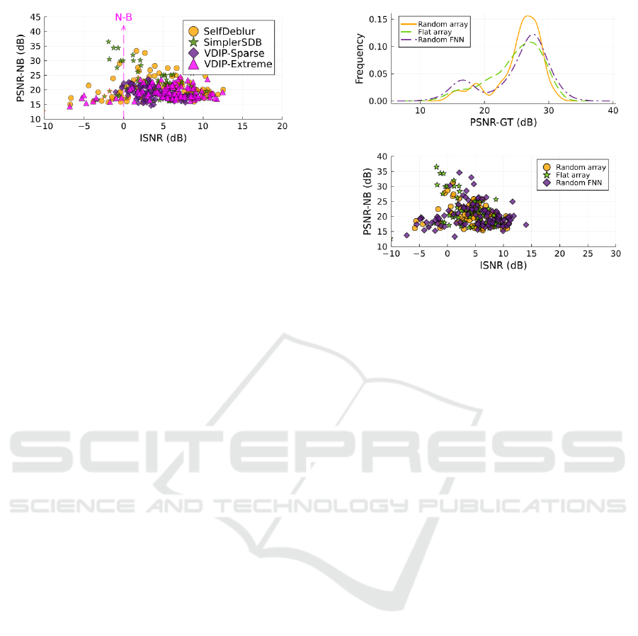
Figure 3: Three runs on the Levin dataset performed
by SelfDeblur, SimplerSDB, VDIP-Sparse, and VDIP-
Extreme. N-B denotes no-blur.
potentially useful information. This is demonstrated
in Figure 2 using the histogram of PSNR (in our pa-
per denoted as PSNR-GT) of the tested algorithms in
their default setup on the Levin dataset. The mean
values of the PSNR are presented in Table 1.
Since the mean value of the SelfDeblur is the high-
est, the conventional ranking procedure would select
it as the best algorithm. While it offers many high-
quality results, it also has many results with very low
PSNR. On the other hand, VDIP-Sparse has almost no
result with PSNR lower than 20 dB, making it a candi-
date with a low risk of poor solution. This advantage
is compensated by the inability to provide excellent
solutions with PSNR greater than 30 dB. An interest-
ing area is around 20 dB PSNR, where VDIP-Extreme
has fewer solutions then SelfDeblur. This motivates
our search for the nature of these results and analyz-
ing which variation of the method influences them.
2.4 Types of Undesired Solutions
The classical literature on BID extensively discusses
two types of undesired solutions: i) the no-blur so-
lution, and ii) an artifact solution. The no-blur so-
lution is an estimate when the image is estimated as
the blurred one, and the PSF as the Dirac delta func-
tion. The loss value of such a solution is zero when
no regularization term is added to (2), so it is cer-
tainly a valid solution, yet undesirable. The artifact
solution is named after visible artifacts corrupting vi-
sually the estimated images. Numerical instability of
DIP, which was observed in the original paper, may
also generate undesirable solutions. These may be
easily detected from the value of the loss function or
prevented by learning rate scheduling.
We will focus our attention only on the no-blur
and artifact solutions. We introduce a modified met-
ric to visualize this distinction. Specifically, we will
compute PSNR not only to the ground truth image,
x
GT
, but also to the blurred image, x
NB
, formally:
PSNR-GT(x) := PSNR(x, x
GT
), (6)
Figure 4: The effect of PSF initilization. Flat and random
array are results obtained by SimplerSDB, random FNN are
generated by SelfDeblur. 3 runs on the Levin dataset.
PSNR-NB(x) := PSNR(x, x
NB
). (7)
The no-blur solutions can be recognized by PSNR-
NB value around 30 dB. Moreover, when comparing
deblurring results on a dataset, it is also useful to mea-
sure the improved signal-to-noise ratio, which is de-
fined as
ISNR(x) = PSNR-GT(x) − PSNR-GT(x
NB
).
Plotting ISNR and PSNR-NB in 2D space, Fig-
ure 3 extends understanding of histogram from Fig-
ure 2. It shows that SelfDeblur and VDIP-Extreme
are prone to solutions with artifacts that are in the area
with low PSNR-NB and negative ISNR. On the other
hand, solutions with ISNR around 0 dB and a high
value of PSNR-NB show that SimplerSDB and Self-
Deblur sometimes reach the no-blur solution. In the
subsequent tests, we analyze which variations of the
studied algorithms influence these solutions.
3 THE NO-BLUR SOLUTION
3.1 Model and Initialization of PSF
Good initialization is an important part of the MAP
approach, such as SelfDeblur. Both the x and k are
initialized randomly. In VDIP, an attempt is made to
pre-train x towards the blurred image (at least con-
tours) and k to a constant array. We now study the
effect of the PSF initialization by various strategies
on the SimplerSDB.
Initialization of k as a constant array was found to
lead to the no-blur solution more likely than initializ-
ing it as a random noise, see Figure 4. On the other
VISAPP 2024 - 19th International Conference on Computer Vision Theory and Applications
562

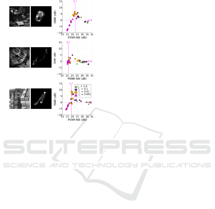
Figure 5: SimplerSDB: Effect of the learning rate η
k
. Each
scatterplot corresponds to deblurring of one image formed
by convolution of the sharp image and the PSF on the left
side. Solid vertical line points in the direction of the ground-
truth, dashed line in the direction of the no-blur.
hand, random noise leads to solutions with artifacts
more often. This holds for both SelfDeblur and Sim-
plerSDB.
Even though neither initialization avoids poor so-
lutions, positive ISNR prevails. We suggest that these
two initializations have similar benefits because their
character is very distinct from the delta function in
the no-blur solution. This hypothesis will be further
developed in the next subsection.
Interestingly, there seems to be no big difference
between modeling k as FNN and σ(θ
k
) only, which
contradicts findings from the original paper (Ren and
et al., 2020).
3.2 The Setting of the Optimizer
In the case of SelfDeblur and SimplerSDB, the setting
of the optimizer plays an important role. We observed
that it is necessary to use the Adam optimizer to reach
a reasonably low loss value. Firstly, LRs influence
whether we find a good, sharp solution or the no-blur
solution.
To see the influence, we deblurred 18 images (4
sharp images from the Levin dataset, 2 from the Ko-
dak dataset (kod, ) blurred by 3 PSFs from the Levin
dataset) with fixed η
x
. Since the best choice of η
k
de-
pends on the blurred image, Figure 5 shows results for
the images separately. It can be seen that higher val-
ues of η
k
lead the algorithm closer to the no-blur solu-
tion. In contrast, too low value of η
k
leads to solutions
with artifacts if the algorithm converges. This behav-
ior is the same for the other tested images. Therefore,
carefully slowing down or speeding up the learning of
k may help to avoid the no-blur solution or solution
with artifacts. We suggest that this is because the ini-
tialization of k is very different from the delta function
and a lower speed of learning of k does not allow the
algorithm to approach the no-blur solution at the be-
ginning of the optimization. On the other hand, with
a higher η
k
, the algorithm descends quickly towards
the no-blur solution, which the DIP should prefer.
Through hyperparameter search we discovered
that increasing the value of β
x
1
(hyperparameter β
1
of
Adam optimiser of x) helps SimplerSDB avoid the
no-blur solution, and the effect is the same for Self-
Deblur. The effect that β
x
1
has on the whole dataset
is shown in Figure 6. We conjecture that this set-
ting helps preserve the original gradient’s momentum
from the initial optimization stages with constant k,
thus avoiding the sharp local minima of the no-blur.
In the case of VDIP, there is no obvious difference for
the two values of β
x
1
, but since VDIP does not gen-
erate any no-blur solutions, it is not that surprising.
3.3 Sharp Image Priors
Undeniably, the most effective way to avoid the no-
blur is the sharp image prior (sparse and extreme
channel) incorporated in the VDIP as can be seen
from Figure 3. The variational Bayesian approach
seems to be important for DIP models since the TV
regularisation did not prove successful (Ren and et al.,
2020; Kotera et al., 2021). Moreover, the VDIP algo-
rithm is not sensitive to the choice of the optimizer
hyperparameters such as β
x
1
studied in Section 3.2.
3.4 Discussion on No-Blur
Mitigation of the no-blur solution has been the objec-
tive of the traditional sharp image priors as well as
various optimization tricks. It is not any different in
the DIP approach. DIP itself does not prefer sharp
images, but carefully setting the optimization hyper-
parameters helps very well to avoid the blurred one.
The best option to avoid the no-blur is the combina-
tion of DIP with a sharp image prior in VDIP.
Avoiding Undesirable Solutions of Deep Blind Image Deconvolution
563

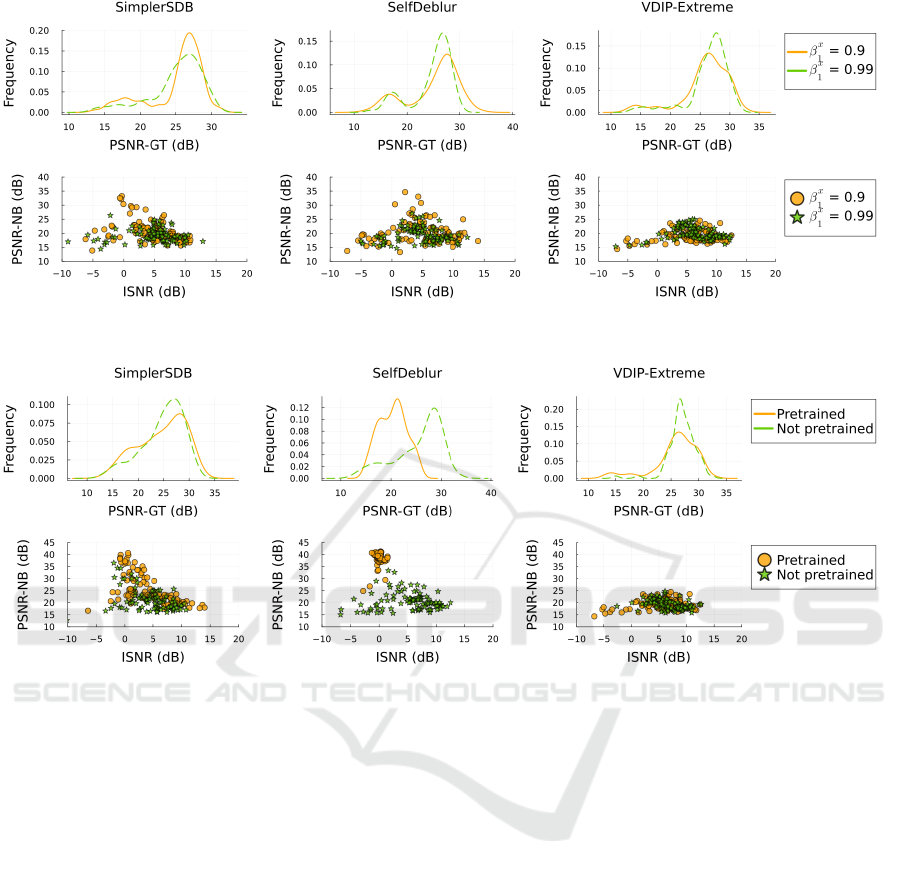
Figure 6: Sensitivity of the solution to the optimizer hyper-parameters β
x
1
in terms of PSNR-NB and ISNR for three runs on
the Levin dataset.
Figure 7: Effect of pretraining on three runs on the Levin dataset.
4 THE ARTIFACT SOLUTION
Solutions with artifacts are generated mostly by Self-
Deblur and VDIP-Extreme.
4.1 Sparse Prior
VDIP-Sparse manages to avoid solutions with arti-
facts, so it can be concluded that the sparse prior min-
imizing differences between neighboring pixels in the
image estimate helps to avoid them. On the other
hand, the prior hinders finding estimates with high
PSNR-GT. The extreme channel prior does not seem
to have this effect.
4.2 Pretraining
VDIP uses pretraining for initialization of both x and
k. G
x
is pretrained to return the blurred image, but
only in 500 iterations, so it learns only the rough con-
tours of the image. The target for k is the constant
array, but after the 500 iterations it still reminds more
of the initial noise. While VDIP-Sparse behaves the
same way when the pretraining is omitted, the per-
formance of VDIP-Extreme improves, and it returns
fewer solutions with artifacts when pretraining is not
used, see Figure 7. The difference could be explained
by the extreme channel prior not being as strong as the
sparse one and getting lost on the trajectory between
the no-blur and sharp solutions.
Since there is no prior in SelfDeblur and Sim-
plerSDB, it could be expected that they will reach
more no-blur solutions when pretrained this way.
Even though SelfDeblur struggles to reach low loss
value, all reconstructions are no-blur solutions. Sim-
plerSDB, on the other hand, does not converge to no-
blur in every run. Considering that the main differ-
ence here is the model of the PSF, the FNN may learn
some information useful for the no-blur during pre-
training, causing all reconstructions to be blurred im-
ages. The optimizers were not reset after pretrain-
ing in this experiment (following how it was done in
VDIP), so the moments used in deblurring were those
learned on a path toward the blurred image. Simply
VISAPP 2024 - 19th International Conference on Computer Vision Theory and Applications
564

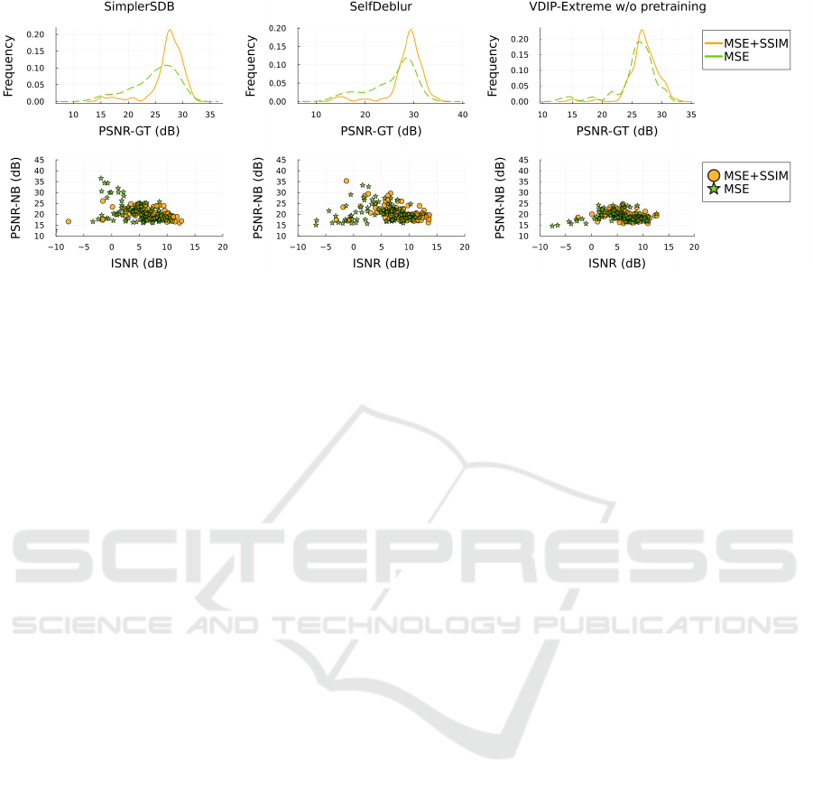
Figure 8: Effect of switching from MSE loss to SSIM loss after 2000 iterations and pretraining on three runs on the Levin
dataset.
loading a new optimizer for deblurring in SelfDeblur
results in a scatterplot quite similar to the one with-
out pretraining and, surprisingly, containing fewer no-
blur solutions. This type of pretraining could work
similarly to lowering the learning rate of the PSF. In
this case, G
x
starts deblurring closer to the solution,
but PSF starts from the same initial point and thus de-
celerates the learning.
4.3 SSIM Loss
Another algorithmic variation used in VDIP (and the
codebase of SelfDeblur) is switching to SSIM loss
(5) after 2000 iterations. Figure 8 shows that VDIP-
Extreme without pretraining requires the use of the
combination of MSE and SSIM loss to avoid solutions
with artifacts. When VDIP-Extreme is pretrained,
there is no significant effect of the switch and it is
the same for VDIP-Sparse (pretrained and not pre-
trained). In the case of SelfDeblur and SimplerSDB,
histograms of PSNR-GT move towards higher val-
ues, but some solutions with artifacts remain. Surpris-
ingly, the no-blur solutions are eliminated in the case
of SimplerSDB. It is difficult to compare these results
because each of these algorithms may be at a different
stage of optimization at the time the loss function is
switched. Overall, the effect of the SSIM loss is sig-
nificant and positive, mostly for the variants without
a sharp image prior.
4.4 Discussion on Artifacts
Artifacts are not visually plausible, making the result-
ing solution undesirable. DIP was proven to prefer
smoother images, so it could be expected to avoid so-
lutions with artifacts and more likely achieve the no-
blur solution. Figure 3 shows that DIP-based models
still reach them, and almost none of the tested vari-
ants avoided them. Even though pretraining could
be expected to push the algorithms towards smoother
solutions, it did not prove to be true. Moreover,
pretraining VDIP-Extreme actually hurts its perfor-
mance. Eventually, the combination of no pretrain-
ing and loss with SSIM helped to get rid of the solu-
tions with artifacts. SSIM loss has a positive effect on
all the tested algorithms, nevertheless, we cannot con-
clude that it helps with the solutions with artifacts ev-
ery time. The only reliable method is the sparse prior
in VDIP-Sparse, which eliminates solutions with ar-
tifacts at the cost of losing excellent solutions with a
lot of details because these images can contain similar
intensity changes as those with artifacts.
5 CONCLUSION
The traditional undesirable solutions of blind image
deconvolution, i.e. the no-blur solution and the so-
lutions with artifacts, are also present in DIP-based
methods. Similarly to the classical methods, the sharp
image prior can effectively avoid the no-blur solution.
In the case of a variation of a DIP method without a
sparse image prior, optimization tricks in the MAP
approach can similarly suppress this solution. The
solution with artifacts, traditionally attributed to in-
versions of poorly conditioned matrices, probably is
not caused only by this numerical inaccuracy and re-
mains a difficult task for DIP-based method as well.
Even though some variations of the method are more
prone to this undesirable solution, such as the switch
to the SSIM metric, a reliable solution still remains to
be found.
Avoiding Undesirable Solutions of Deep Blind Image Deconvolution
565

ACKNOWLEDGEMENTS
This work was supported by the grants GA20-27939S
and GA24-10400S.
REFERENCES
Kodak image datset. http://r0k.us/graphics/kodak/. Ac-
cessed: 2020-01-13.
Asim, M., Shamshad, F., and Ahmed, A. (2020). Blind im-
age deconvolution using deep generative priors. IEEE
Trans Comput Imaging, 6:1493–1506.
Babacan, S. D., Molina, R., and Katsaggelos, A. K. (2009).
Variational bayesian blind deconvolution using a total
variation prior. IEEE Trans Image Process, 18(1):12–
26.
Bredell, G., Erdil, E., Weber, B., and Konukoglu, E. (2023).
Wiener guided dip for unsupervised blind image de-
convolution. In 2023 IEEE/CVF WACV, pages 3046–
3055.
Chan, T. and Wong, C.-K. (1998). Total variation blind de-
convolution. IEEE Trans Image Process, 7(3):370–
375.
Huang, Y., Chouzenoux, E., and Pesquet, J.-C. (2023). Un-
rolled variational bayesian algorithm for image blind
deconvolution. IEEE Trans Image Process, 32:430–
445.
Huo, D., Masoumzadeh, A., Kushol, R., and Yang, Y.-H.
(2023). Blind image deconvolution using variational
deep image prior. IEEE Trans Pattern Anal Mach In-
tell, 45(10):11472–11483.
Kingma, D. P. and Ba, J. (2014). Adam: A
method for stochastic optimization. arXiv preprint
arXiv:1412.6980.
Kotera, J.,
ˇ
Sm
´
ıdl, V., and
ˇ
Sroubek, F. (2017). Blind decon-
volution with model discrepancies. IEEE Trans Image
Process, 26(5):2533–2544.
Kotera, J.,
ˇ
Sroubek, F., and
ˇ
Sm
´
ıdl, V. (2021). Improving
neural blind deconvolution. In 2021 IEEE ICIP, pages
1954–1958. IEEE.
Levin, A., Weiss, Y., Durand, F., and Freeman, W. T. (2009).
Understanding and evaluating blind deconvolution al-
gorithms. In 2009 IEEE CVPR, pages 1964–1971.
Levin, A., Yair, W., Fredo, D., and Freeman, W. T. (2011).
Understanding blind deconvolution algorithms. IEEE
Trans Pattern Anal Mach Intell, 33(12):2354–2367.
Likas, A. C. and Galatsanos, N. P. (2004). A variational ap-
proach for bayesian blind image deconvolution. IEEE
Trans Signal Process, 52(8):2222–2233.
Miskin, J. and MacKay, D. J. C. (2000). Ensemble learn-
ing for blind image separation and deconvolution. In
Advances in Independent Component Analysis, pages
123–141. Springer, London, 1 edition.
Molina, R., Mateos, J., and Katsaggelos, A. K. (2006).
Blind deconvolution using a variational approach to
parameter, image, and blur estimation. IEEE Trans
Image Process, 15(12):3715–3727.
Perrone, D. and Favaro, P. (2016). A clearer picture of to-
tal variation blind deconvolution. IEEE Trans Pattern
Anal Mach Intell, 38(6):1041–1055.
Ren, D. and et al. (2020). Neural blind deconvolution us-
ing deep priors. In 2020 IEEE/CVF CVPR, pages pp.
3338–3347. IEEE.
Ronneberger, O., Fischer, P., and Brox, T. (2015). U-
net: Convolutional networks for biomedical image
segmentation. In MICCAI 2015, pages 234–241.
Springer, Cham, 1. edition.
Shi, Z., Mettes, P., Maji, S., and Snoek, C. G. (2022). On
measuring and controlling the spectral bias of the deep
image prior. International Journal of Computer Vi-
sion, 130:885–908.
Shin, C. J., Lee, T. B., and Heo, Y. S. (2021). Dual im-
age deblurring using deep image prior. Electronics,
10(17).
Tzikas, D., Likas, A., and Galatsanos, N. (2009). Varia-
tional bayesian sparse kernel-based blind image de-
convolution with student’s-t priors. IEEE Trans Image
Process, 18(4):753–764.
Ulyanov, D., Vedaldi, A., and Lempitski, V. (2018). Deep
image prior. In 2018 IEEE/CVF CVPR, pages 9446–
9454. IEEE.
Wang, Z., Bovik, A., Sheikh, H., and Simoncelli, E. (2004).
Image quality assessment: from error visibility to
structural similarity. IEEE Trans Image Process,
13(4):600–612.
Wang, Z., Wang, Z., Li, Q., and Bilen, H. (2019). Image
deconvolution with deep image and kernel priors. In
2019 IEEE/CVF ICCVW, pages 980–989.
Wipf, D. and Zhang, H. (2014). Revisiting bayesian blind
deconvolution. Journal of Machine Learning Re-
search, 15:3775–3814.
Yan, Y., Ren, W., Guo, Y., Wang, R., and Cao, X. (2017).
Image deblurring via extreme channels prior. In 2017
IEEE CVPR, pages 6978–6986.
Zhao, Q., Wang, H., Yue, Z., and Meng, D. (2022). A
deep variational bayesian framework for blind image
deblurring. Knowledge-Based Systems, 249.
VISAPP 2024 - 19th International Conference on Computer Vision Theory and Applications
566