Data-Driven Viscosity Solver for Fluid Simulation

Wonjung Park

, Hyunsoo Kim

and Jinah Park

Korea Advanced Institute of Science and Technology, Daejeon, Korea

Keywords:

Physical Simulation, Machine Learning, Viscous Fluid, Convolutional Neural Network.

Abstract:

We propose a data-driven viscosity solver based on U-shaped convolutional neural network to predict velocity

changes due to viscosity. Our solver takes velocity derivatives, ﬂuid volume, and solid indicator quantities

as input. The traditional marker-and-cell (MAC) grid stores velocities at the edges of the grid, causing the

dimensions of the velocity ﬁeld vary from axis to axis. In our work, we suggest a symmetric MAC grid

that maintains consistent dimensions across axes without interpolation or symmetry breaking. The proposed

grid effectively transfers spatial ﬂuid quantities such as partial derivatives of velocity, enabling networks to

generate accurate predictions. Additionally, we introduce a physics-based loss inspired by the variational

formulation of viscosity to enhance the network’s generalization for a wide range of viscosity coefﬁcients.

We demonstrate various ﬂuid simulation results, including 2D and 3D ﬂuid-rigid body scenes and a scene

exhibiting the buckling effect.

1 INTRODUCTION

Numerical methods for ﬂuid simulation have been

widely used in various ﬁelds such as industrial design,

and computer graphics. These methods solve incom-

pressible Navier-Stokes (N-S) equations, the govern-

ing equation of ﬂuid dynamics in the form of partial

differential equations (PDEs). The process of solving

N-S equations is well-known for being computation-

ally expensive and the cost is mostly from solving a

series of linear systems by iterative methods.

In recent years, various studies (Kim et al., 2019;

Richter-Powell et al., 2022; Tompson et al., 2017)

have adopted machine learning to accelerate the pro-

jection step of ﬂuid simulation. By replacing iterative

methods with highly parallel GPU-optimized neural

networks, they were able to greatly accelerate the

overall ﬂuid simulation. In addition to the parallelism,

these methods exploit the fact that pressure makes the

ﬂuid incompressible. Unlike typical machine learning

regression, which solely relies on supervised learning

from the dataset, they are designed to enforce the in-

compressibility of the velocity ﬁeld. Therefore, they

can be trained with a small dataset and generalize well

to scenes outside of the training data.

Although the data-driven projection solver accel-

https://orcid.org/0000-0003-1075-612X

https://orcid.org/0000-0002-0404-1892

https://orcid.org/0000-0003-4676-9862

erates the simulation of inviscid ﬂuid to the real-time

level, we found that it is insigniﬁcant when used for

a viscous ﬂuid. Traditional viscosity solvers have to

solve linear systems that are 4 times larger than the

projection stage in 2D (x8 for 3D), since it deals with

twice more ﬂuid quantities per each dimension. How-

ever, studies on the data-driven viscosity solver have

not yet been conducted in depth, since generalization

of the viscosity solver is a challenging problem.

The challenge comes from two factors. First, it

is difﬁcult for networks to generalize over viscosity

coefﬁcients because it varies in a wide range from

zero (inviscid) to inﬁnity (solid). Second, the pressure

is stored at the cell center whereas the ﬂuid velocity

is stored at the cell boundary of the marker-and-cell

(MAC) grid for Eulerian simulation. This structure

yields an asymmetry of the velocity ﬁeld; for exam-

ple, the velocity of the x-direction has the dimension

(n + 1,n) but the y-direction has (n,n +1) for the Eu-

lerian MAC grid n × n. Therefore, unlike general im-

age data for CNNs, ﬂuid velocity requires special care

due to their distinct and asymmetric structure.

We design the viscosity solver architecture with

these problems in mind. To generalize the solver

for viscosity coefﬁcients, we inherit the variational

interpretation of the viscosity from the conventional

solver (Batty and Bridson, 2008), using its minimiza-

tion problem as the training loss. In addition, we in-

troduce the symmetric MAC grid to enable the sym-

Park, W., Kim, H. and Park, J.

Data-Driven Viscosity Solver for Fluid Simulation.

DOI: 10.5220/0012397300003660

Paper published under CC license (CC BY-NC-ND 4.0)

In Proceedings of the 19th International Joint Conference on Computer Vision, Imaging and Computer Graphics Theory and Applications (VISIGRAPP 2024) - Volume 1: GRAPP, HUCAPP

and IVAPP, pages 269-276

ISBN: 978-989-758-679-8; ISSN: 2184-4321

269

metric representation of ﬂuids regardless of the axis.

To our knowledge, this is the ﬁrst data-driven vis-

cosity solver, so we focus on elaborating an archi-

tecture that generalizes to various scenarios. In this

paper, we validate our architecture through ablation

studies of neural network conﬁgurations. Finally, we

demonstrate the universality of our solver in various

scenarios, including unseen rigid-ﬂuid scenes, mixed

dynamic viscosity scenes, and 3D scene which shows

buckling effect of viscous ﬂuid.

2 RELATED WORK

The main subject of this study is to simulate viscous

ﬂuids governed by the incompressible Navier-Stokes

(N-S) equations with our data-driven viscosity solver.

The Navier-Stokes (N-S) equations are:

= −

∇p +

∇

v + g, (1)

∇ · v = 0. (2)

There are three approaches to numerically simulate

the N-S equations: grid-based (Eulerian), particle-

based (Lagrangian), and Lagrangian/Eulerian hybrid

appraoches. Hybrid simulation uses particles to trans-

port ﬂuid and grids to update velocity by external

forces, pressure, and viscosity. For spatial discretiza-

tion of ﬂuid quantities, marker-and-cell method (Har-

low and Welch, 1965), which stores velocities on

edges of cells, is often used in grid-based simulation.

The projection term in the N-S equations (the

ﬁrst term in the RHS of Equ. 1) enforces the incom-

pressibility as formulated in Equ. 2. Combining the

two equations gives Poisson’s equation (∇

p = f ),

whose discrete form can be solved using linear sys-

tem solvers.

The viscosity term in the N-S equations (second

term in RHS of Equ. 1) gives the viscous behavior,

accounting for internal friction. With explicit solvers,

this term can become numerically unstable especially

for high dynamic viscosity µ. Thus, a more stable

implicit formulation of the viscosity ﬂuid for hybrid

methods is proposed in (Batty and Bridson, 2008).

They interpreted the viscosity term as a minimization

problem that seeks to minimize the rate of viscous dis-

sipation with the smallest velocity change possible. In

2D, the minimization problem is deﬁned as:

min

−→



−→

u −

−→

old



+2∆t



∇

−→

u + (∇

−→

u )

)



(3)

To reduce the computational cost of ﬂuid simula-

tions, various dimensionality reduction methods have

been proposed. Model reduction for ﬂuid-rigid sim-

ulation is discussed in (Treuille et al., 2006). In ad-

dition, multi-resolution Eulerian grids are introduced

for efﬁcient Poisson equation solving in both invis-

cid (Chentanez and M

uller, 2011; McAdams et al.,

2010) and viscous ﬂuids (Aanjaneya et al., 2019;

Shao et al., 2022). Furthermore, recent studies ap-

plied machine learning techniques including princi-

pal component analysis (Xiao et al., 2018b), regres-

sion forests (Ladick

y et al., 2015), Long Short-Term

Memory (Wiewel et al., 2020), generative adversar-

ial networks (Cheng et al., 2020), and graph net-

works (Sanchez-Gonzalez et al., 2020; Li and Fari-

mani, 2022).

Among these machine learning techniques, con-

volutional neural networks (CNNs) have shown their

effectiveness in Eulerian and hybrid ﬂuid simulation.

Since the Eulerian grid has a similar structure to the

image, many studies applied CNN to ﬂuid simulation

(Guo et al., 2016; Obiols-Sales et al., 2020; Thuerey

et al., 2020; Xiao et al., 2019). Some studies (Kim

et al., 2019) proposed generative networks that out-

put the next velocity ﬁelds based on reduced param-

eters. Alternatively, other studies (Tompson et al.,

2017; Xiao et al., 2018b; Xiao et al., 2018a; Yang

et al., 2016; Gao et al., 2020) maintain the traditional

ﬂuid simulation process but replace the most time-

consuming projection step with a data-driven solver.

The traditional projection step with discretized PDE is

computationally expensive and data dependent, since

it is solved by iterative methods until it meets the con-

ditions. Thus, the replacement of Poisson’s equation

with deep learning techniques (Richter-Powell et al.,

2022; Tang et al., 2017) have been actively researched

to efﬁciently derive the solution. Despite the efﬁ-

ciency and generalization of these data-driven projec-

tion solvers, their impact on viscous ﬂuids is limited

as the viscosity step remains a signiﬁcant bottleneck.

In this study, we propose a CNN-based viscos-

ity solver that replaces the PDE-based solver (Batty

and Bridson, 2008) to effectively reduce the compu-

tational costs of the viscous ﬂuid.

3 METHOD

3.1 Data-Driven Viscosity Solver

We suggest a data-driven viscosity solver that predicts

velocity change by viscosity. As Fig. 1 shows, the

overall process is based on the afﬁne particle-in-cell

(APIC) (Jiang et al., 2015) simulator, which trans-

ports ﬂuid with particles and updates the velocity by

external force, viscosity, and pressure on the grid. The

GRAPP 2024 - 19th International Conference on Computer Graphics Theory and Applications

270

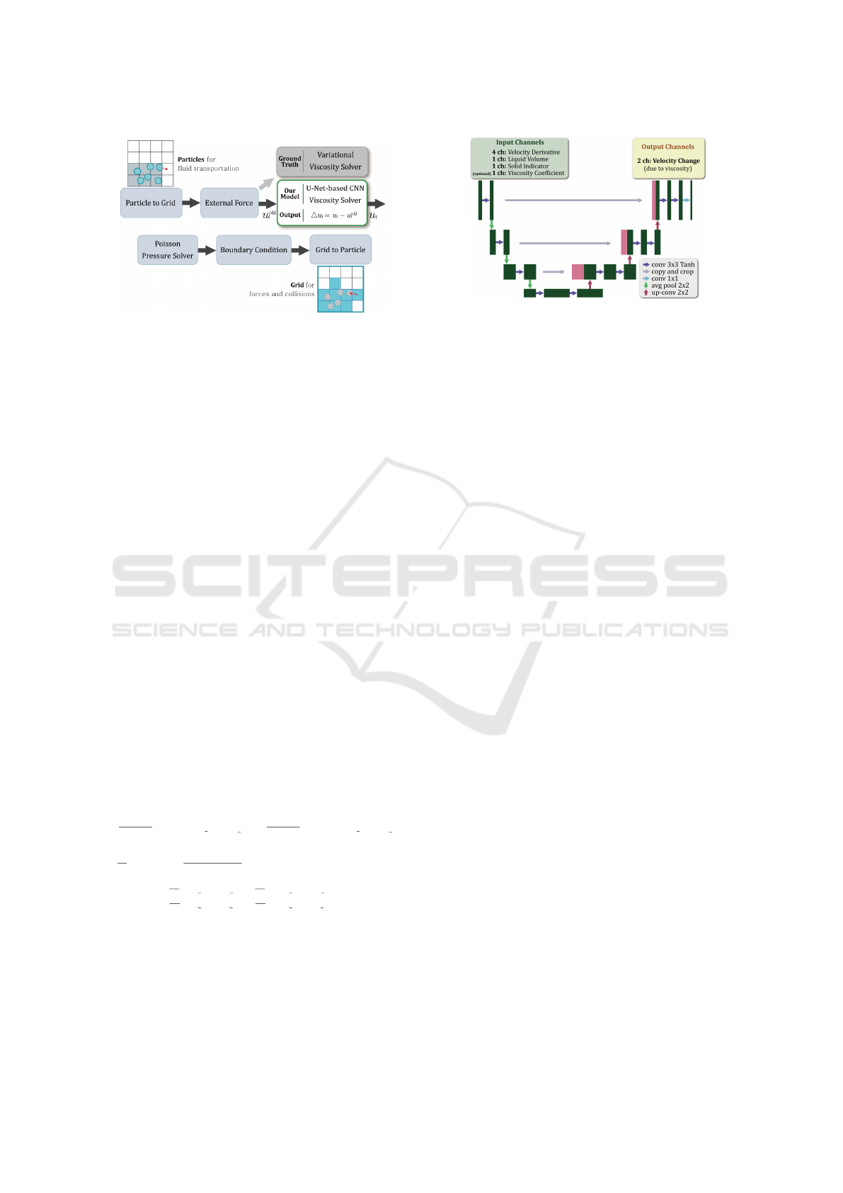
Figure 1: Fluid simulation with data-driven viscosity

solver. Using the traditional afﬁne particle-in-cell (Jiang

et al., 2015) simulator as a baseline, our data-driven solver

replaces the viscosity solver to output velocity changes due

to viscosity. Training ground truth is generated with the tra-

ditional viscosity solver (Batty and Bridson, 2008).

viscosity solver updates the velocity u

old

from the ex-

ternal force step (gravity) to the velocity u

. We use

the velocity difference △u

= u

− u

old

solved by the

traditional solver (Batty and Bridson, 2008) as the

ground truth for training.

3.1.1 Loss Function

We train our model by supervised learning with L2

loss which is the mean squared error between ground

truth and model output. In addition, we suggest the

variational loss L

which is the variational formula-

tion of the conventional viscosity solver. When train-

ing the model only for ﬁxed dynamic viscosity, L2

loss is sufﬁcient to converge the model. However, for

a dataset that contains various dynamic viscosity at

the same time, we use both losses together to regu-

larize the network for dynamic viscosity µ. Our loss

function is composed of the sum of L2 loss and varia-

tional loss L

with equal weights. We trained the net-

work with Adam optimizer(Kingma and Ba, 2014).

The variational loss L

on the 2D Eulerian grid is de-

rived as follows, where velocity u = (u,v):

(u,△t,ρ,µ)

n(n + 1)

n+1

∑

i=1

∑

j=1



i−

, j

−u

old

i−

, j



n(n + 1)

∑

i=1

n+1

∑

j=1



i, j−

−v

old

i, j−



2△t

∑

i=1

∑

j=1



(▽u

i, j

+ ▽u

i, j

)



where ▽u

i, j

△x

, j

−u

i−

, j

)

△y

i, j+

−u

i, j−

)

△x

, j

−v

i−

, j

)

△y

i, j+

−v

i, j−

)

(4)

The sum of the ﬁrst and second term of L

can be

derived by the average of the element-wise squared

output because the output is velocity change due to

viscosity. The third term denotes the ﬂuid dissipa-

tion over the timestep. Through this term, L

im-

poses a greater loss for higher viscosity, helping the

Figure 2: U-Shaped convolutional neural network for our

data-driven viscosity solver.

network to create less velocity difference between ad-

jacent ﬂuid elements.

3.2 Architecture

3.2.1 u-Shaped CNN Model

We design the neural network architecture with the

following two conditions in mind. First, the network

allows input and output to have the same dimensions

in width and height since they are deﬁned on the same

Eulerian grid. Second, the architecture should grasp

important features of viscosity.

Viscosity is the resistance force of a ﬂuid that re-

duces the velocity difference with neighboring ﬂuids.

In addition, ﬂuids in the boundary layer, which is a

thin layer near the boundary between the ﬂuid and the

solid, are more affected by viscosity. In other words,

both the local feature representing adjacent ﬂuid ele-

ments and the global feature revealing the location of

the ﬂuid element with respect to the ﬂuid-rigid body

scene are important for predicting the velocity. There-

fore, we set the U-Net (Ronneberger et al., 2015) as

a backbone because its multi-resolution feature maps

help the network learn both local and global features

of ﬂuid-rigid body scene, and generate output of the

same size as the input.

Unlike the image segmentation task of the orig-

inal U-Net, our viscosity solver aims to output the

velocity change for each dimension. The velocity

change has the distinct property that it has the range

(−∞,∞). Constructing a network that produces exact

velocity changes that could be positive or negative is

a challenging task. To ﬁnd the best architecture, we

have experimented with various conditions to explore

which model predicts accurate and unbiased output.

As a result, our network consists of tangent hyper-

bolic activation function and average pooling layers

as depicted in Fig. 2. We will elaborate the compari-

son of network conﬁguration in section 4.

Data-Driven Viscosity Solver for Fluid Simulation

271

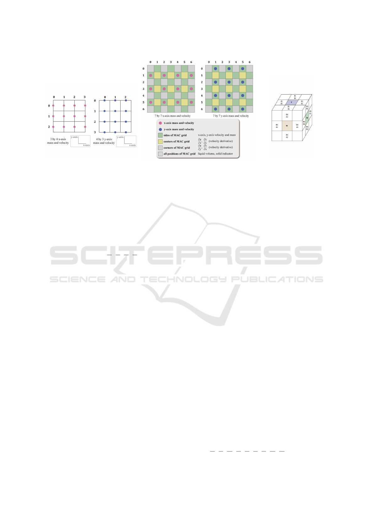
(a) Marker-and-cell (MAC) grid. (b) Symmetric MAC grid for 2D CNN. (c) Symmetric MAC grid for 3D CNN.

Figure 3: Extension of the MAC grid for CNN-based viscosity solver To adjust input channel dimensions without losing

information or breaking symmetry, we propose the symmetric MAC grid. This grid ensures symmetry in all input channels.

3.2.2 Conﬁguration of Input Channels

Our data-driven solver takes all necessary ﬂuid quan-

tities as input. This includes velocity derivatives to

capture velocity differences with neighboring grid po-

sitions. In addition, the conventional solver requires

ﬂuid volume for each cell and a phase indicator (solid

or not) on the grid positions. In summary, for the

2D grid, the input channels consist of four veloc-

ity derivative channels

∂u

∂x

∂v

∂y

∂u

∂y

∂v

∂x

for the velocity

ﬁeld u = (u,v), one channel for ﬂuid volume, and one

channel for the solid indicator.

Velocity Derivative Channels. We use velocity

derivatives instead of velocity itself in the construc-

tion of input channels because viscosity acts to re-

duce the velocity derivatives of the neighboring ﬂuid.

Moreover, using the velocity itself as input, the output

would be varied by the velocity scale. For example,

during free fall, there should be no velocity change

caused by viscosity, but the network prones to output

varying values due to the accelerated velocity. Hence,

velocity derivative channels are employed for gener-

alization across different velocity scales.

Fluid Volume Channel. To convey the volume quan-

tity to the CNN, we suggest using a ﬂuid volume

channel. First, the signed distance from the ﬂuid sur-

face, constructed from a spherical surface of each par-

ticle, is computed for each corner (4 corners for 2D

cell, and 8 for 3D cell) of the cell. From signed dis-

tances of two adjacent corner d

and d

−

, edge occu-

pancy of ﬂuid is derived as V

= −(d

−

/(d

− d

−

)).

Then, the face (or volume) occupancy is approxi-

mated as the average of the occupancy of its 4 edges

(or 6 faces in 3D). For the generalization of the ﬂuid

volume, we normalized the volume by the factor of

maximum volume of one grid cell, so that the ﬂuid

volume is in [0, 1].

Solid Indicator Channel. In addition, to deliver the

status of the grid position, we suggest solid indicator

channel, constructed by the signed distance D

i, j

from

solid on the position x = (i, j). We set the solid indi-

cator channel as follows:

solid indicator

i, j



0 if D

i, j

> 0

1 if D

i, j

≤ 0

(5)

Viscosity Coefﬁcient Channel. Finally, we suggest

an optional viscosity coefﬁcient channel. While the

network converges well without this channel when

trained for a ﬁxed viscosity coefﬁcient, it becomes es-

sential for generalization across a wide range of vis-

cosity coefﬁcients. The viscosity coefﬁcient channel,

denoted by coeff

i, j

, is assigned the dynamic viscosity

µ in Pa·s. When implementing the channel, only cells

with positive ﬂuid volume are set as µ. The viscosity

coefﬁcient channel is set as follows:

coeff

i, j



0 if cell

i, j

is air or solid

µ if cell

i, j

is liquid

(6)

The U-shaped architecture requires pooling, thus

we expand the dimension by padding to be divisible

by 2

where n is the number of pooling layers. Zero

padding is applied for velocity derivative, ﬂuid vol-

ume, and viscosity coefﬁcient channels, while one is

used for a solid indicator channel. Random padding

is applied to both the height and width dimensions to

accommodate the various positions of the rigid body.

Our architecture readily extends to 3D ﬂuid

simulation using the symmetric MAC grid for 3D

ﬂuid quantities as shown in Fig. 3c. All layers

of U-shaped architecture should be replaced into

3D layers, for example, 3D convolution, 3D av-

erage pooling, and 3D transposed convolution lay-

ers for upsampling. The input channels are given

with

∂u

∂x

∂v

∂y

∂w

∂z

∂u

∂y

∂u

∂z

∂v

∂x

∂v

∂z

∂w

∂x

∂w

∂y

, ﬂuid volume,

GRAPP 2024 - 19th International Conference on Computer Graphics Theory and Applications

272

and solid indicator on symmetric MAC grid for ﬂuid

velocity u = (u,v,w).

3.3 Symmetric MAC Grid for CNN

Marker-and-cell (MAC) grid (Harlow and Welch,

1965) stores ﬂuid velocity and mass quantities at the

edge of the grid as illustrated in Fig. 3(a) so that the

dimensions of the quantities vary from axis to axis.

For example, for the grid size (n,n), the velocity di-

mension of the x-direction is (n + 1, n) and the y-

direction is (n,n +1). Therefore, to input information

from the x and y-direction together, modifying the di-

mensions is required.

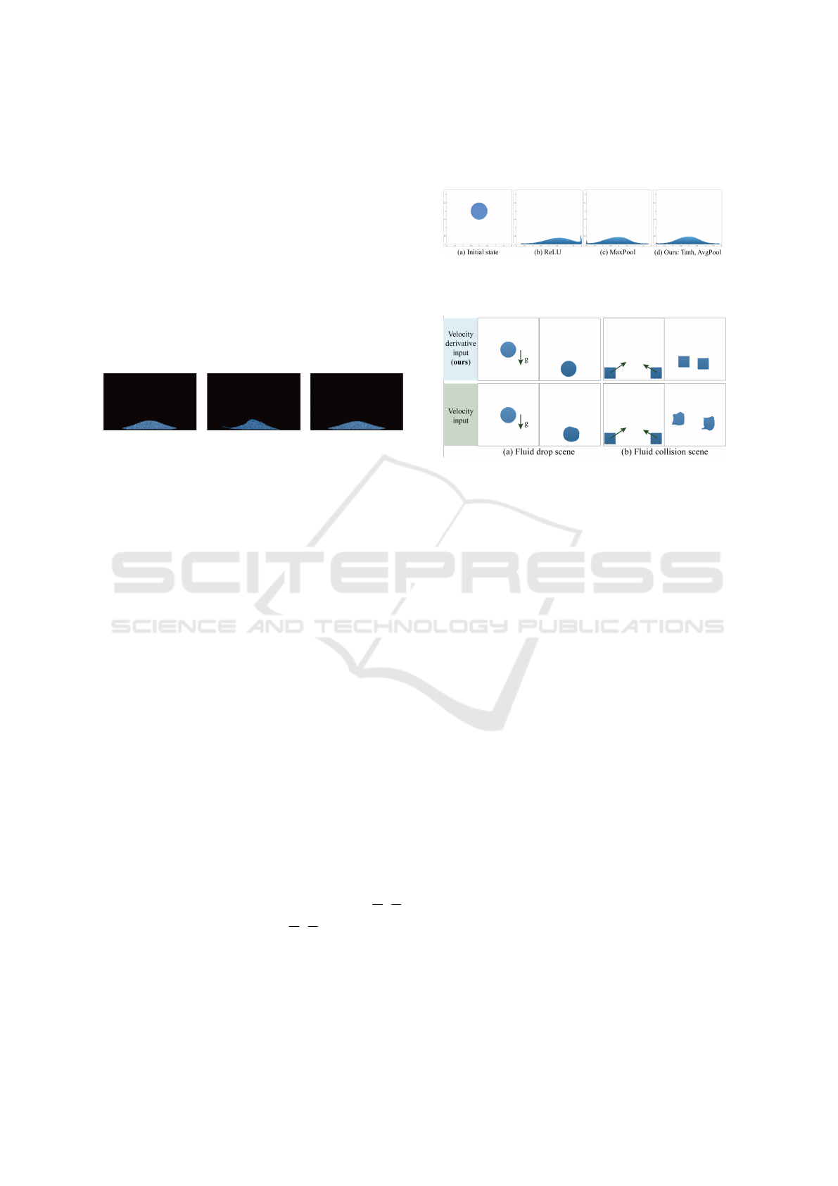
Figure 4: Comparison of input architecture. (Left)

Ground truth, (Middle) Result from the input with simple

padding, and (Right) input with our symmetric MAC grid.

For ﬂuid simulation, ﬂuid quantities must be han-

dled with care since tiny biases accumulate errors

over successive frames. For the case of CNN for im-

ages, interpolation or padding could be a simple so-

lution that rectiﬁes the dimension. However, interpo-

lation yields a loss of ﬂuid information. Furthermore,

simple padding causes an asymmetry between input

channels that results in a tilted simulation, as Fig. 4

illustrates.

To address this problem we suggest a symmet-

ric MAC grid for CNN that preserves all information

without loss and generates symmetric input channels,

regardless of the axis. Our symmetric MAC grid ex-

tends the original MAC grid including not only the

centers but also the corners and edges of the cells.

Therefore, the dimension of the symmetric MAC grid

becomes (2n + 1, 2n + 1) for the (n,n) grid. The

quantities of mass and velocity of the x-direction are

deﬁned in pink circles, and the y-direction in blue cir-

cles as shown in Fig. 3(b). The network output chan-

nels, which are the x-direction and the y-direction ve-

locity change, are also placed in the same position.

The other cells without value are ﬁlled with zero not

to inﬂuence the neural network.

In addition, this architecture facilitates the genera-

tion of derivative channels. To be more speciﬁc,

∂u

∂x

∂v

∂y

are placed in the yellow cell and

∂u

∂y

∂v

∂x

are in the gray

cell. Liquid volume and solid indicator channels are

calculated for all cells. Therefore, our input architec-

ture guarantees that all input channels are symmetric

and yields symmetric simulation results as shown in

Fig. 4.

4 EXPERIMENTS ON U-SHAPED

CNN ARCHITECTURE

Figure 5: (a) From the initial resting state, the frame with

(b) average pooling and ReLU (c) max pooling and tangent

hyperbolic (Tanh) (d) average pooling and Tanh (ours).

Figure 6: Top row: velocity derivative input and Bottom

row: velocity input for (a) ﬂuid drop and (b) colliding ﬂuids

scenes. The scenes are in a training dataset.

Ablation studies on network architecture are demon-

strated in this section. We verify our network for vari-

ous conditions including activation functions, pooling

methods, and input channels.

Activation Function and Pooling Layers. The most

important factor in network conﬁguration is unbiased

learning because bias results in tilted simulation. To

explore the best CNN layers, we conducted abla-

tion studies for the activation function between ReLU

and tangent hyperbolic, and the pooling method be-

tween the max and average pooling. As shown in

Fig. 5, ReLU which removes negative features, and

max pooling layer which ignores small features pro-

duce a distorted result for ﬂuid drop scene. Therefore,

we design our network with a tangent hyperbolic ac-

tivation function and average pooling layers.

Velocity Channel vs. Velocity Derivative Channel.

As mentioned in subsubsection 3.2.2, the network re-

ceives velocity derivatives instead of raw velocity in-

puts. As shown in Fig. 6(a), the velocity derivative

maintains the shape of the sphere during free fall,

whereas the velocity channel distorts the sphere. This

is because the velocity is accelerated, so the CNN

solver prones to produce different outputs across the

time steps. On the other hand, since the velocity

derivative has a constant value of zero during free fall,

the consistent output is generated. For the same rea-

son, the velocity channel also produces a strange be-

havior for a more dynamic scene such as Fig. 6(b).

Data-Driven Viscosity Solver for Fluid Simulation

273

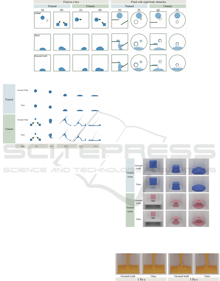
Figure 7: Simulation result comparison between our data-driven solver and ground truth for various scenarios.

Figure 8: Simulation result comparison with timestamps for

both trained and unseen scenes.

5 RESULTS

5.1 Universality of Data-Driven

Viscosity Solver

In order to verify the universality of the proposed ar-

chitecture, we demonstrate ﬂuid simulation with var-

ious scenarios: ﬂuids in a box, ﬂuids with rigid body

obstacles, and 3D scenes exhibiting buckling effect.

5.1.1 Viscous Fluid with Rigid Bodies

We demonstrate our solver with two scenarios: ﬂuid

in a box and ﬂuid with rigid body obstacles in Fig. 7.

Both scenes are constructed with 1 Pa·s dynamic

viscosity, 300 Hz framerate, 2m × 2m space, and

100 × 100 Eulerian grid dimension. The training

epoch is 2000 and the learning rate is 5 × 10

−4

. Our

data-driven viscosity solver (with four pooling layers)

takes approximately 0.007 seconds per frame.

For the ﬂuid in a box scenario, the neural net-

work is trained using 5-second ﬂuid simulations of

Fig. 7(a,b), resulting in a dataset consisting of 1500

frames for each scene. Our solver outputs acceptable

visual ﬁdelity for both trained and unseen(Fig. 7(c,d))

scenarios.

We tested our method in more complex scenes

with rigid body obstacles. The network is trained with

10-seconds ﬂuid simulations of Fig. 7(e,f). Our solver

also shows similar results to ground truth for unseen

scenes of Fig. 7(g,h).

For further validation of our data-driven simula-

tion, we performed a timestamp-based comparison

between ours and the ground truth. For both trained

and unseen scenarios, our data-driven solver con-

sistently predicts similar velocity changes for every

timestamp as visualized in Fig. 8.

Figure 9: 3D ﬂuid-rigid simulation Trained solely on the

ﬂuid drop scene, our solver similarly simulates the unseen

scene with the ground truth. The space is 2m × 2m × 2m

with 80 × 80 × 80 Eulerian grid dimension.

Figure 10: Buckling effect of viscous ﬂuid with 1 and 5

Pa·s dynamic viscosities. The simulated space is 0.6m ×

1m × 0.6m with Eulerian grid dimension 48 × 80 × 48.

GRAPP 2024 - 19th International Conference on Computer Graphics Theory and Applications

274

5.1.2 Extension to 3D Fluid Simulation

As depicted in Fig. 9, our solver trained on a ﬂuid

drop scene successfully performs 3D ﬂuid simula-

tions for both trained and unseen scenes. The net-

work effectively learns viscosity characteristics using

data from a simple scene and extends its capability in

more complex scenes with rigid bodies.

Our viscosity solver (with two pooling layers)

takes approximately 0.39 seconds per frame with an

80 × 80 × 80 Eulerian grid for scenes in Fig. 9.

Moreover, our solver simulates the buckling effect

of viscous ﬂuid, demonstrated in Fig. 10. Similar to

the ground truth, the ﬂuid with a lower viscosity co-

efﬁcient (1 Pa·s) exhibits reduced buckling compared

to the 5 Pa·s case.

5.2 Generalization of Dynamic Viscosity

Figure 11: (a) Fluid drop scenes with one neural network

model for various viscosity coefﬁcients.(b) Simulation re-

sult with viscosity coefﬁcient channel set by left side as

1000 and right side as 1 mPa·s.

Our network can be generalized to various dynamic

viscosities µ. To provide dynamic viscosity informa-

tion, the viscosity coefﬁcient input channel is option-

ally given to the network as mentioned in subsubsec-

tion 3.2.2. U-shaped viscosity solver with four pool-

ing layers is trained by 12000 frames consisting of

dynamic viscosity 1, 100, 500, 1000, 2000, and 3000

mPa·s equally. The trained model is well generalized

for unseen coefﬁcients as shown in Fig. 11(a). For ex-

ample, although 700 mPa·s is not learned, it is spread

narrower than 100 and wider than 3000.

However, as shown in Fig. 11, our data-driven

solver cannot extrapolate the viscosity simulations

outside the trained dynamic viscosity range. The sim-

ulation is tilted to the right and upside because a large

dynamic viscosity affects the network to output large

x-direction (right) and y-direction (upward) velocity

changes. Therefore, a corresponding dataset is re-

quired to generate the model for a wide range of dy-

namic viscosity.

Moreover, mixed dynamic viscosity can be simu-

lated without additional training. For example, we as-

signed dynamic viscosity 1000 to the left and 1 mPa·s

to the right side in Fig. 11(b). The left side is less

spread out due to the large viscosity, whereas the right

side ﬂuid spreads like water. We anticipate that our

model can be applied to complex scenes with multiple

viscosity coefﬁcients. In-depth exploration of multi-

ple viscosity coefﬁcients remains a future work.

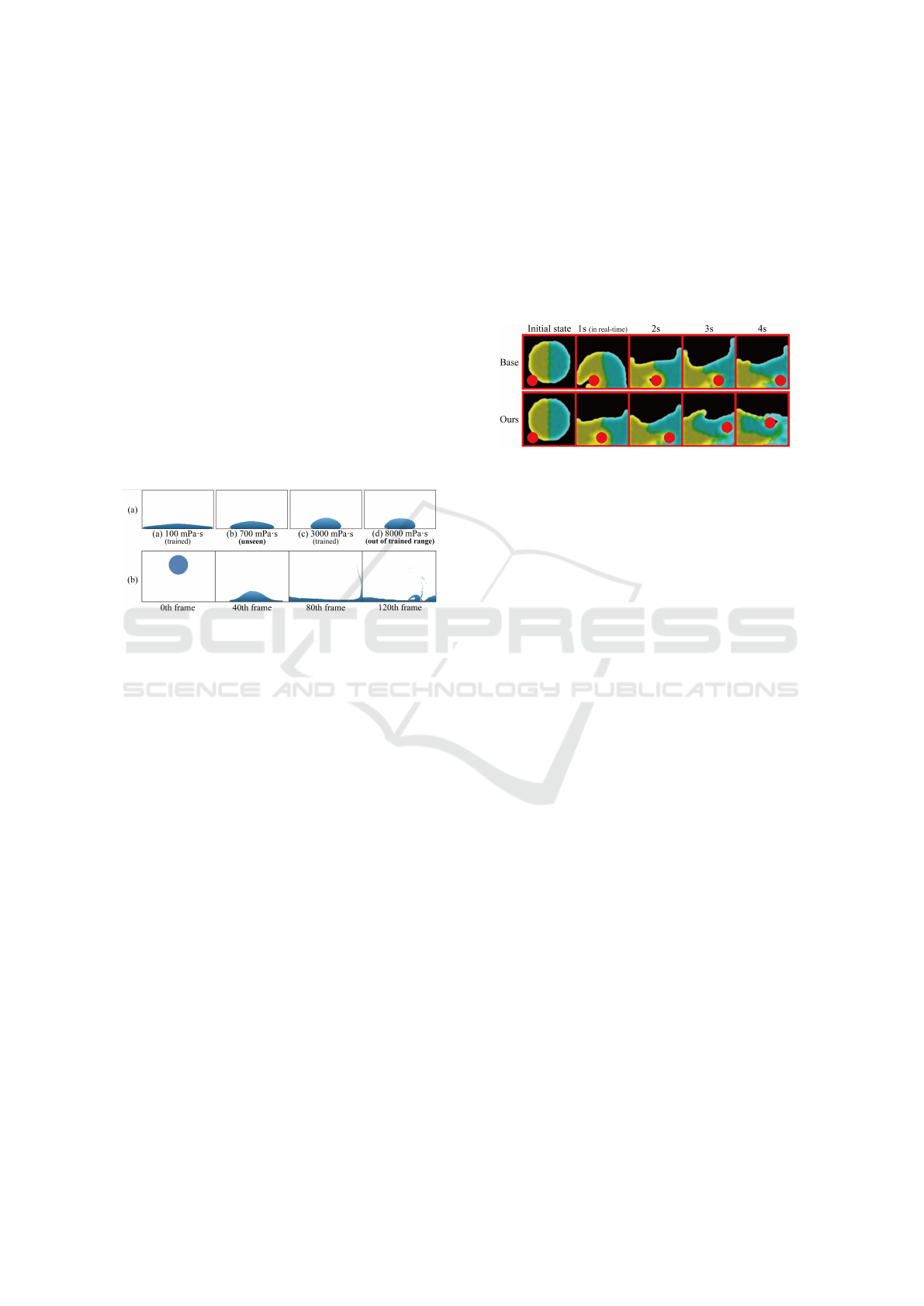
5.3 Real-Time Application of

Rigid-Fluid Interaction

Figure 12: Progression of real-time 2D rigid-ﬂuid interac-

tive application. Top row: Iterative viscosity solver (Batty

and Bridson, 2008). Bottom row: Our U-shaped CNN vis-

cosity solver which is nearly twice faster.

To demonstrate the efﬁciency of our solver, we ap-

plied our solver to a real-time interactive application

of paint mixing Fig. 12 where a rigid pointer (red cir-

cle) perturbs ﬂuid of two different colors. The scene

consists of (25, 25) grid dimension and 848 particles.

On average, the baseline (Batty and Bridson, 2008)

runs at 14 Hz (71 ms) with 32ms iterative viscosity

solver, and ours takes 23Hz (42 ms) with 4ms data-

driven viscosity solver.

6 CONCLUSION

In this paper, we propose a data-driven viscosity

solver for a hybrid Lagrangian/Eulerian ﬂuid simu-

lator, utilizing a symmetric MAC grid to represent

ﬂuid quantities without symmetry breaking or inter-

polation. Our U-shaped CNN, with input channels of

velocity derivatives, ﬂuid volume, and solid indica-

tors, predicts velocity changes with reasonable error

in both trained and unseen scenes. To show the effec-

tiveness of our architecture, we demonstrate various

scenes, including ﬂuid with rigid bodies, mixed dy-

namic viscosity, and 3D ﬂuid with a buckling effect.

We believe that the proposed data-driven viscos-

ity solver can be utilized for diverse ﬂuid simulation,

as demonstrated in a real-time interactive application.

Our solver’s generalizability across a wide viscosity

range is achieved through a viscosity coefﬁcient chan-

nel and a physics-based variational loss. While we

primarily analyze our network in 2D space, we plan

to further explore and optimize our method for 3D

viscous ﬂuid simulation.

Data-Driven Viscosity Solver for Fluid Simulation

275

ACKNOWLEDGEMENTS

This work was supported by Institute for Informa-

tion & communications Technology Promotion(IITP)

grant funded by the Korea government(MSIT)

(No.00223446, Development of object-oriented syn-

thetic data generation and evaluation methods).

REFERENCES

Aanjaneya, M., Han, C., Goldade, R., and Batty, C. (2019).

An efﬁcient geometric multigrid solver for viscous

liquids. Proceedings of the ACM on Computer Graph-

ics and Interactive Techniques, 2(2):1–21.

Batty, C. and Bridson, R. (2008). Accurate viscous

free surfaces for buckling, coiling, and rotating liq-

uids. In In Proc. Symposium on Computer Anima-

tion.ACM/Eurographics, page 219–228.

Cheng, M., Fang, F., Pain, C. C., and Navon, I. (2020).

Data-driven modelling of nonlinear spatio-temporal

ﬂuid ﬂows using a deep convolutional generative ad-

versarial network. Computer Methods in Applied Me-

chanics and Engineering, 365:113000.

Chentanez, N. and M

uller, M. (2011). Real-time eulerian

water simulation using a restricted tall cell grid. In

ACM Siggraph 2011 Papers, pages 1–10.

Gao, Y., Zhang, Q., Li, S., Hao, A., and Qin, H. (2020).

Accelerating liquid simulation with an improved data-

driven method. In Computer Graphics Forum, vol-

ume 39, pages 180–191. Wiley Online Library.

Guo, X., Li, W., and Iorio, F. (2016). Convolutional neural

networks for steady ﬂow approximation. In Proceed-

ings of the 22nd ACM SIGKDD international confer-

ence on knowledge discovery and data mining, pages

481–490.

Harlow, F. H. and Welch, J. E. (1965). Numerical calcu-

lation of time-dependent viscous incompressible ﬂow

of ﬂuid with free surface. The physics of ﬂuids,

8(12):2182–2189.

Jiang, C., Schroeder, C., Selle, A., Teran, J., and Stomakhin,

A. (2015). The afﬁne particle-in-cell method. ACM

Transactions on Graphics (TOG), 34(4):1–10.

Kim, B., Azevedo, V. C., Thuerey, N., Kim, T., Gross, M.,

and Solenthaler, B. (2019). Deep ﬂuids: A generative

network for parameterized ﬂuid simulations. In Com-

puter graphics forum, volume 38, pages 59–70. Wiley

Online Library.

Kingma, D. P. and Ba, J. (2014). Adam: A

method for stochastic optimization. arXiv preprint

arXiv:1412.6980.

Ladick

y, L., Jeong, S., Solenthaler, B., Pollefeys, M., and

Gross, M. (2015). Data-driven ﬂuid simulations us-

ing regression forests. ACM Transactions on Graphics

(TOG), 34(6):1–9.

Li, Z. and Farimani, A. B. (2022). Graph neural network-

accelerated lagrangian ﬂuid simulation. Computers &

Graphics, 103:201–211.

McAdams, A., Sifakis, E., and Teran, J. (2010). A parallel

multigrid poisson solver for ﬂuids simulation on large

grids. In Symposium on Computer Animation, pages

65–73.

Obiols-Sales, O., Vishnu, A., Malaya, N., and Chan-

dramowliswharan, A. (2020). Cfdnet: A deep

learning-based accelerator for ﬂuid simulations. In

Proceedings of the 34th ACM international confer-

ence on supercomputing, pages 1–12.

Richter-Powell, J., Lipman, Y., and Chen, R. T. (2022).

Neural conservation laws: A divergence-free perspec-

tive. arXiv preprint arXiv:2210.01741 (2022).

Ronneberger, O., Fischer, P., and Brox, T. (2015). U-net:

Convolutional networks for biomedical image seg-

mentation. In International Conference on Medical

image computing and computer-assisted intervention,

pages 234–241. Springer.

Sanchez-Gonzalez, A., Godwin, J., Pfaff, T., Ying, R.,

Leskovec, J., and Battaglia, P. (2020). Learning to

simulate complex physics with graph networks. In

International conference on machine learning, pages

8459–8468. PMLR.

Shao, H., Huang, L., and Michels, D. L. (2022). A fast un-

smoothed aggregation algebraic multigrid framework

for the large-scale simulation of incompressible ﬂow.

ACM Transactions on Graphics (TOG), 41(4):1–18.

Tang, W., Shan, T., Dang, X., Li, M., Yang, F., Xu, S.,

and Wu, J. (2017). Study on a poisson’s equation

solver based on deep learning technique. In 2017

IEEE Electrical Design of Advanced Packaging and

Systems Symposium (EDAPS), pages 1–3.

Thuerey, N., Weißenow, K., Prantl, L., and Hu, X. (2020).

Deep learning methods for reynolds-averaged navier–

stokes simulations of airfoil ﬂows. AIAA Journal,

58(1):25–36.

Tompson, J., Schlachter, K., Sprechmann, P., and Perlin,

K. (2017). Accelerating eulerian ﬂuid simulation with

convolutional networks. In International Conference

on Machine Learning, pages 3424–3433. PMLR.

Treuille, A., Lewis, A., and Popovi

c, Z. (2006). Model

reduction for real-time ﬂuids. ACM Transactions on

Graphics (TOG), 25(3):826–834.

Wiewel, S., Kim, B., Azevedo, V. C., Solenthaler, B., and

Thuerey, N. (2020). Latent space subdivision: sta-

ble and controllable time predictions for ﬂuid ﬂow. In

Computer Graphics Forum, volume 39, pages 15–25.

Wiley Online Library.

Xiao, X., Wang, H., and Yang, X. (2019). A cnn-based

ﬂow correction method for fast preview. In Computer

Graphics Forum, volume 38, pages 431–440. Wiley

Online Library.

Xiao, X., Yang, C., and Yang, X. (2018a). Adaptive

learning-based projection method for smoke simula-

tion. Computer Animation and Virtual Worlds, 29(3-

4):e1837.

Xiao, X., Zhou, Y., Wang, H., and Yang, X. (2018b).

A novel cnn-based poisson solver for ﬂuid simula-

tion. IEEE transactions on visualization and computer

graphics, 26(3):1454–1465.

Yang, C., Yang, X., and Xiao, X. (2016). Data-driven pro-

jection method in ﬂuid simulation. Computer Anima-

tion and Virtual Worlds, 27(3-4):415–424.

GRAPP 2024 - 19th International Conference on Computer Graphics Theory and Applications

276