Investigating the Corruption Robustness of Image Classiﬁers with

Random p-norm Corruptions

Georg Siedel

1,2

, Weijia Shao

, Silvia Vock

and Andrey Morozov

Federal Institute for Occupational Safety and Health (BAuA), Dresden, Germany

University of Stuttgart, Germany

Keywords:

Image Classiﬁcation, Corruption Robustness, p-norm.

Abstract:

Robustness is a fundamental property of machine learning classiﬁers required to achieve safety and reliability.

In the ﬁeld of adversarial robustness of image classiﬁers, robustness is commonly deﬁned as the stability of a

model to all input changes within a p-norm distance. However, in the ﬁeld of random corruption robustness,

variations observed in the real world are used, while p-norm corruptions are rarely considered. This study

investigates the use of random p-norm corruptions to augment the training and test data of image classiﬁers.

We evaluate the model robustness against imperceptible random p-norm corruptions and propose a novel

robustness metric. We empirically investigate whether robustness transfers across different p-norms and derive

conclusions on which p-norm corruptions a model should be trained and evaluated. We ﬁnd that training data

augmentation with a combination of p-norm corruptions signiﬁcantly improves corruption robustness, even

on top of state-of-the-art data augmentation schemes.

1 INTRODUCTION

State-of-the-art computer vision models achieve

human-level performance in various tasks, such as

image classiﬁcation (Krizhevsky et al., 2017). This

makes them potential candidates for challenging vi-

sion tasks. However, they tend to be easily fooled by

small changes in their input data, which limits their

overall dependability to perform in safety-critical ap-

plications (Carlini and Wagner, 2017). For classiﬁca-

tion models, robustness against small data changes is

therefore considered a fundamental pillar of AI de-

pendability and has attracted considerable research

interest in recent years.

Within the robustness research landscape, the ad-

versarial robustness domain has received the most at-

tention (Drenkow et al., 2021). An adversarial attack

aims to ﬁnd worst-case counterexamples for robust-

ness. However, vision models are not only vulnerable

to small worst-case data manipulations in the input

data but also to randomly corrupted input data (Dodge

and Karam, 2017). Accordingly, the corruption ro-

bustness

domain aims at models that perform sim-

ilarly well on data corrupted with random noise. A

clear distinction needs to be made between adversar-

Also called statistical robustness

Figure 1: Samples drawn uniformly in 2D from a L

0.5

and

a L

norm sphere (left and right) and a L

and a L

norm

ball (middle).

ial robustness and corruption robustness: Existing re-

search suggests that these two types of robustness tar-

get different model properties and applications (Wang

et al., 2021). Also, adversarial robustness and cor-

ruption robustness do not necessarily transfer to each

other, and adversarial robustness is much harder to

achieve in high-dimensional input space (Fawzi et al.,

2018a; Ford et al., 2019).

1.1 Motivation

The adversarial robustness domain provides the clear-

est deﬁnition of robustness based on a maximum ma-

nipulation distance in the p-norm space (see Section

2.1) (Drenkow et al., 2021). Accordingly, there exists

a set of p-norms and maximum distances ε for each

norm that are commonly used for robustness evalua-

tion on popular image classiﬁcation benchmarks, e.g.

Siedel, G., Shao, W., Vock, S. and Morozov, A.

Investigating the Corruption Robustness of Image Classiﬁers with Random p-norm Corruptions.

DOI: 10.5220/0012397100003660

Paper published under CC license (CC BY-NC-ND 4.0)

In Proceedings of the 19th International Joint Conference on Computer Vision, Imaging and Computer Graphics Theory and Applications (VISIGRAPP 2024) - Volume 2: VISAPP, pages

171-181

ISBN: 978-989-758-679-8; ISSN: 2184-4321

171

∞

with ε = 8/255 and L

with ε = 0.5 on the CI-

FAR and SVHN benchmark datasets (Croce and Hein,

2020; Yang et al., 2020).

In contrast, corruption robustness is commonly as-

sessed by testing data corruptions originating from

camera, hardware, or environment (Hendrycks and

Dietterich, 2019). Such data corruptions can occur

in real-world applications

. Investigating robustness

using p-norm distances is rarely employed in the cor-

ruption robustness domain. We present three argu-

ments to motivate our investigation into this area.

First of all, the adversarial robustness targets the

signiﬁcant performance degradation caused by p-

norm manipulations that are small or, even worse, im-

perceptible (Carlini and Wagner, 2017; Szegedy et al.,

2013; Zhang et al., 2019). From our point of view, a

classiﬁer should generalize in line with human per-

ception, regardless of whether the manipulations are

adversarial or random. Therefore, we want to inves-

tigate whether the same is true for random p-norm

corruptions.

Second, related work has shown that increasing

the range of training data augmentations can improve

the performance of classiﬁers (Mintun et al., 2021;

uller and Hutter, 2021). Therefore, we expect that

combining different p-norm corruptions at training

time will lead to effective robustness improvements.

Furthermore, studies have shown the difﬁculty

of predicting transferability among different types of

corruption (Hendrycks and Dietterich, 2019; Ford

et al., 2019). Given the large differences between the

volumes covered by different p-norm balls in high-

dimensional space (see Table 6 in the appendix), we

suspect the same for different p-norm corruptions,

which should be observable in the empirical evalua-

tion.

1.2 Contributions

This paper investigates image classiﬁers trained and

tested on random p-norm corruptions.

The main

contributions can be summarized as follows:

• We test classiﬁers on random quasi-imperceptible

corruptions from different p-norms and demon-

strate a performance degradation. We propose to

measure this minimum requirement for corruption

robustness with a corresponding robustness met-

ric.

• We present an empirically effective training data

augmentation strategy based on combinations of

thus we refer to them as ”real-world corruptions”, even

though they are usually artiﬁcially created

Code available: https://github.com/Georgsiedel/Lp-

norm-corruption-robustness

p-norm corruptions that improve robustness more

effectively than individual corruptions.

• We evaluate how robustness obtained from train-

ing on p-norm corruptions transfers to other p-

norm corruptions and to real-world corruptions.

We discuss the transfer of p-norm corruption ro-

bustness from a test coverage perspective.

2 PRELIMINARIES

2.1 Robustness Deﬁnition

A classiﬁer g is locally robust at a data point x within

a distance ε > 0, if g(x) = g(x

′

) holds for all perturbed

points x

′

that satisfy

dist(x,x

′

) ≤ ε (1)

with x

′

close to x according to a predeﬁned distance

measure (Carlini and Wagner, 2017).

In the adversarial attack domain (Carlini and Wag-

ner, 2017), this distance in R

is commonly induced

by a p-norm (Weng et al., 2018; Yang et al., 2020),

for 0 ≤ p ≤ ∞

∥x −x

′

∥

= (

∑

i=1

− x

′

)

1/p

. (2)

2.2 Sampling Algorithm

In order to experiment with random corruptions uni-

formly distributed within a p-norm ball or sphere, an

algorithm that scales to high-dimensional space is re-

quired for all norms 0 < p < ∞

. We use the approach

in (Calaﬁore et al., 1998), which is described in detail

in the Appendix.

Figure 1 visualises samples for different p-norm

unit balls in R

using the proposed algorithm, demon-

strating its ability to sample uniformly inside the ball

and on the sphere.

3 RELATED WORK

p-norm Distances in the Robustness Context. As

described in Section 2.1, p-norm distances are used to

deﬁne adversarial robustness. Furthermore, p-norm

distances have been used to measure certain proper-

ties of image data related to robustness. One such

Here, we abuse the term ”norm distance” by also using

0 ≤ p < 1, which are no norms by mathematical deﬁnition.

p = 0 (set a ratio ε of dimensions to 0 or 1) and p = ∞

(add uniform random value from [ε, −ε] to every dimen-

sion) are trivial from a sampling perspective.

VISAPP 2024 - 19th International Conference on Computer Vision Theory and Applications

172

property is the threshold at which an image manip-

ulation is imperceptible, which is a reference point

in the ﬁeld of adversarial robustness (Szegedy et al.,

2013). L

∞

manipulations with ε = 8/255 have been

used in conjunction with the imperceptibility thresh-

old (Zhang et al., 2019; Madry et al., 2017). How-

ever, it is difﬁcult to justify an exact imperceptibil-

ity threshold (Zhang et al., 2019). Researchers have

therefore called for further research into ”distance

metrics closer to human perception” (Huang et al.,

2020). There exist similarity measures for images

that are more aligned with human perception than p-

norm distances (Wang et al., 2004). To the best of

our knowledge, these measures have not yet been used

as distance measures for the robustness evaluation of

perception models.

Another property of image data measured using

p-norm distances in the context of robustness is the

class separation of a dataset. The average class sep-

aration is used by (Fawzi et al., 2018b) in order to

obtain a comparable baseline distance for robustness

testing. Similarly, (Yang et al., 2020) measure the

minimum class separation on typical image classiﬁ-

cation benchmarks using L

∞

-distances. The authors

conclude the existence of a perfectly robust classiﬁer

with respect to this distance. Building on this idea,

(Siedel et al., 2022) investigate robustness on random

∞

-corruptions with minimum class separation dis-

tance, obtaining an interpretable robustness metric.

(Wang et al., 2021) test and train image classi-

ﬁers on data corrupted by few random L

∞

corruptions.

Overall, little research has been directed at using ran-

dom corruptions based on p-norm distances to evalu-

ate robustness.

Real-World Data Corruptions for Testing. In com-

parison, much research uses real-world corruptions to

evaluate robustness, such as the popular benchmark

by (Hendrycks and Dietterich, 2019) and extensions

thereof like in (Mintun et al., 2021).

Real-World Data Corruptions for Training. Real-

world data corruptions are also used as training data

augmentations alongside geometric transformations

in order to obtain better generalizing or more robust

classiﬁers (Shorten and Khoshgoftaar, 2019). Some

training data augmentations only target accuracy but

not robustness (Cubuk et al., 2020; M

uller and Hut-

ter, 2021). A few approaches use only geometric

transformations, such as cuts, translations and rota-

tions, to improve overall robustness (Yun et al., 2019;

Hendrycks et al., 2019). Some approaches make use

of random noise, such as Gaussian and Impulse noise,

to improve robustness (Lopes et al., 2019; Dai and

Berleant, 2021; Lim et al., 2021; Erichson et al.,

2022).

Even though accuracy and robustness have long

been considered as an inherent trade-off (Tsipras

et al., 2019; Zhang et al., 2019). Several described

data augmentation methods manage to increase cor-

ruption robustness along with accuracy (Hendrycks

et al., 2019; Lopes et al., 2019). Some data aug-

mentation methods even leverage random corruptions

to implicitly or explicitly improve or give guarantees

for adversarial robustness (Cohen et al., 2019; Weng

et al., 2019; Lecuyer et al., 2019; Yun et al., 2019).

Classic Noise and p-norm Corruptions. Some per-

turbation techniques used in signal processing are

closely related to p-norm corruptions. Gaussian noise

shares similarities with L

-norm corruptions (Cohen

et al., 2019). Impulse Noise or Salt-and-Pepper Noise

are similar to this paper’s notion of L

-norm corrup-

tions. Applying brightness or darkness to an image

is a non-random L

∞

corruption that applies the same

change to every pixel. This similarity further moti-

vates our investigation of the behaviour of various p-

norm corruptions.

Robustness Transferability. Robustness is typically

speciﬁc to the type of corruption or attack the model

was trained for. Adversarial or corruption robustness

is only to a limited extent transferable between each

other (Fawzi et al., 2018a; Fawzi et al., 2018b; Rusak

et al., 2020), across different p-norm attacks and at-

tack strengths (Carlini et al., 2019), or across real-

world corruption types (Hendrycks and Dietterich,

2019; Ford et al., 2019). This ﬁnding motivates our

investigation into whether random p-norm corruption

robustness transfers to other p-norm corruptions and

real-world corruptions.

Wide Training Data Augmentation. Recent efforts

suggest that choosing randomly from a wide range

of augmentations can be more effective compared to

more sophisticated augmentation strategies (Mintun

et al., 2021; M

uller and Hutter, 2021). Furthermore,

(Kireev et al., 2022) ﬁnd that training with single

types of noise overﬁts with regards to both noise type

and noise level. These results encourage us to investi-

gate the combination of training time p-norm corrup-

tions that effectively improve corruption robustness.

4 EXPERIMENTAL SETUP

4.1 Robustness Metrics

In addition to the standard test error E

clean

, we use 4

metrics to assess the corruption robustness of all our

trained models. For all reported metrics, low values

indicate a better performance.

To cover well-known real-world corruptions, we

Investigating the Corruption Robustness of Image Classiﬁers with Random p-norm Corruptions

173

Figure 2: Examples from the chosen set of imperceptible

corruptions on CIFAR (above) and TinyImageNet (below).

compute the mCE (mean Corruption Error) metric

using the benchmark by (Hendrycks and Dietterich,

2019). We use a 100% error rate as a baseline, so that

mCE corresponds to the average error rates E across

19 different corruptions c and 5 corruption severities

s each:

mCE = (

∑

s=1

∑

c=1

s,c

)/(5 ∗ 19) (3)

We additionally report mCE without the 4 noise cor-

ruptions included in the metric, which we denote

mCE

(mean Corruption Error ex Noise). This met-

ric evaluates robustness against the remaining 15 cor-

ruption types that are not based on any form of pixel-

wise noise, such as the p-norm corruptions we train

on. To cover random p-norm corruptions, we intro-

duce a robustness metric mCE

(mean Corruption

Error p-norm), which is calculated similarly as (3)

from the average of the error rates. As shown in

Table 1, the corruptions c for mCE

are 9 differ-

ent p-norms and the severities s are 10 different ε-

values for each p-norm. The p-norms and ε-values

were manually selected to cover a wide range of val-

ues and to lead to signiﬁcant and comparable perfor-

mance degradation of a standard model.

In order to investigate imperceptible random p-

norm corruptions, we propose the iCE (imperceptible

Corruption Error) metric:

iCE = (

∑

i=1

− E

clean

)/(n ∗ E

clean

), (4)

where n is the number of different imperceptible cor-

ruptions. This metric can be considered as a mini-

mum requirement for the corruption robustness of a

classiﬁer. iCE quantiﬁes the increase in error rate rel-

ative to the clean error rate E

clean

and is therefore ex-

pressed in %. For each dataset in our study, we choose

n = 6 p-norm corruptions (Table 1). We select p and

ε-values based on a small set of randomly sampled

and maximally corrupted images. Figure 2 visualizes

such corruptions compared to the original image for

the CIFAR and TinyImageNet datasets.

Table 1: Sets of p-norm corruptions for calculating the

mCE

and iCE metrics. Brackets contain the minimum

and maximum out of 10 ε-values for each p-norm. For L

ε is the ratio of maximally corrupted image dimensions.

p mCE

[ε

min

,ε

max

] iCE [ε]

CIFAR TIN CIFAR TIN

0 [0.005, 0.12] [0.01, 0.3]

0.5 [2.5e+4, 4e+5] [2e+5, 1.2e+7] 2.5e+4 7e+5

1 [12.5, 200] [37.5, 1500] 25 125

2 [0.25, 5] [0.5, 20] 0.5 2

5 [0.03, 0.6] [0.05, 1.5]

10 [0.02, 0.3] [0.02, 0.7] 0.03 0.06

50 [0.01, 0.18] [0.02, 0.35] 0.02 0.04

200 [0.01, 0.15] [0.02, 0.3]

∞ [0.005, 0.15] [0.01, 0.3] 0.01 0.01

4.2 Training Setup

Experiments are performed on the CIFAR-10 (C10),

CIFAR-100 (C100) (Krizhevsky et al., 2009) and

Tiny ImageNet (TIN) (Le and Yang, 2015) classiﬁ-

cation datasets. We train 3 architectures of convolu-

tional neural networks: A WideResNet28-4 (WRN)

with 0.3 dropout probability (Zagoruyko and Ko-

modakis, 2016), a DenseNet201-12 (DN) (Huang

et al., 2017) and a ResNeXt29-32x4d (RNX) (Xie

et al., 2017) model. We use a Cosine Annealing

Learning Rate schedule with 150 epochs and an ini-

tial learning rate of 0.1, restarting after 10, 30 and 70

epochs (Loshchilov and Hutter, 2016). As an opti-

mizer, we use SGD with 0.9 momentum and 0.0005

learning rate decay. We use a batch size of 384, resize

the image data to the interval [0,1] and augment with

random horizontal ﬂips and random cropping.

In addition to standard training, we apply a

set of p-norm corruptions to the training dataset,

each with different ε-values. The norms used are

0.5

and L

∞

. L

(40) denotes a model

trained exclusively on data augmented with L

cor-

ruptions with ε ≤ 40. We manually selected the set

of p-norms to cover a wide range of values and the 2

ε-values for each p-norm so that we observe a mean-

ingfully large effect on the metrics for all p-norms.

We also train with combinations of p-norm cor-

ruptions by randomly applying one from a wider set

of p-norm corruptions and ε-values. An overview of

the 3 different combined corruption sets is shown in

Table 2, denoted C1, C2 and C3. We apply a p-norm

corruption sample to a minibatch of 8 images during

training. This avoids computational drawbacks of cal-

culating the sampling algorithm for 0 < p < ∞ on the

CPU, resulting in almost no additional overhead.

Furthermore, the p-norm corruption combinations

are compared and combined with the 4 state-of-the-art

VISAPP 2024 - 19th International Conference on Computer Vision Theory and Applications

174

Table 2: Sets of p-norm corruptions for the training of the

models C1, C2 and C3. Brackets contain the minimum and

maximum out of 10 (C1 and C2) or 5 (C3) ε-values for each

p-norm.

p [ε

min

, ε

max

]

C1 C2 C3 on CIFAR C3 on TIN

0 + + [0.005, 0.03]∗ [0.01, 0.075]∗

0.5 + [2.5e+4, 1.5e+5∗ [2e+5, 1.8e+6]∗

1 + [12.5, 75]∗ [37.5, 300]∗

2 + + [0.25, 1.5]∗ [0.5, 4]∗

5 + [0.03, 0.2]∗ [0.05, 0.3]∗

10 + [0.02, 0.1]∗ [0.02, 0.14]∗

50 + [0.01, 0.06]∗ [0.02, 0.1]∗

200 + [0.01, 0.05]∗ [0.02, 0.08]∗

∞ + + [0.005, 0.04]∗ [0.01, 0.06]∗

+ Same ε-values as in mCE

for this p-norm (see Table 1

∗ Lowest 5 of the 10 ε-values in mCE

for this p-norm

(see Table 1)

data augmentation and mixing strategies TrivialAug-

ment (TA) (M

uller and Hutter, 2021), RandAug-

ment (RA) (Cubuk et al., 2020) and AugMix (AM)

(Hendrycks et al., 2019) and Mixup (MU) (Zhang

et al., 2018). Accordingly, TA+C1 denotes a model

trained on images with TA augmentation followed by

the C1 corruption.

5 RESULTS

Table 3 compares different models trained with p-

norm corruptions on the CIFAR-100 dataset with re-

spect to the metrics described above. The table shows

that all corruption-trained models produce improved

mCE and mCE

values at the expense of clean ac-

curacy. Increasing the intensity of training corrup-

tions mostly increases this effect. L

training is an

exception where this effect is inconsistent. We ﬁnd

that there is a much smaller positive effect of cor-

ruption training on mCE

. For corruption training

outside of L

, increasing the intensity of corruptions

actually worsens mCE

. The combined corruption

models C1, C2 and C3 achieve much higher improve-

ments in robustness than the models trained on one

corruption only, with a similar degradation of clean

accuracy. In particular, they achieve signiﬁcantly im-

proved mCE

robustness. Model C2 performs better

than C1 overall. C3 achieves slightly lower robust-

ness to noise (mCE and mCE

), but better clean ac-

curacy. The standard model and the models trained

on L

corruptions show signiﬁcant iCE values, while

iCE is close to zero for all other models.

Table 4 illustrates the effect of a selection of train-

Table 3: All metrics for the DenseNet model on CIFAR-

100. We compare standard training data with various p-

norm corrupted training data and combinations of p-norm

corrupted training data.

Model E

clean

mCE mCE

mCE

iCE

Standard 23.21 51.33 46.19 53.70 12.41%

(0.01) 24.08 47.32 45.76 45.57 8.6%

(0.03) 23.62 47.24 44.80 47.25 7.7%

0.5

(7.5e+4) 25.86 47.91 45.83 41.22 -1.0%

0.5

(1.5e+5) 26.35 43.11 44.15 33.83 -0.1%

(50) 25.68 47.78 45.11 41.86 -1.0%

(100) 29.12 45.64 46.28 34.12 -0.1%

(1) 24.77 48.92 45.71 44.06 0.0%

(2.5) 28.98 46.33 46.39 35.11 -0.4%

(0.03) 24.82 48.67 45.27 44.87 -0.7%

(0.08) 28.95 47.02 46.68 36.39 -0.5%

∞

(0.02) 25.05 48.63 45.47 43.79 -0.6%

∞

(0.04) 28.89 47.69 47.04 37.41 -0.2%

C1 27.51 39.66 41.85 29.67 0.8%

C2 26.04 39.31 41.75 28.38 0.9%

C3 24.60 40.30 41.73 29.88 0.7%

ing time p-norm corruptions and combined corrup-

tions. To generalise the results, we report the delta

of all metrics with the standard model, averaged over

all model architectures. The table shows that L

cor-

ruption training slightly increases robustness, with the

least negative impact on clean accuracy on the CIFAR

datasets at the same time. The L

0.5

corruption training

is the most effective among the single corruptions to

increase mCE and mCE

. The L

∞

corruption training

is the least effective in terms of the ratio of robustness

gained per clean accuracy lost. In fact, on the Tiny

ImageNet dataset, no single p-norm corruption train-

ing signiﬁcantly reduces either mCE or mCE

. On

all datasets, C1, C2 and C3 achieve the most signiﬁ-

cant robustness improvements. C3 stands out partic-

ularly on Tiny ImageNet, where it is the only model

that improves clean accuracy while effectively reduc-

ing mCE or mCE

Figure 3 illustrates how the robustness obtained

from training on different single p-norm corruptions

transfers to robustness against other p-norm corrup-

tions. It shows that L

corruptions are a special case.

Training on L

corruptions gives the model very high

robustness against L

corruptions, but less robustness

against all other p-norm corruptions compared with

other training strategies. At the same time, no p-norm

corruption training except L

effectively achieves ro-

bustness against L

corruptions. Except for the L

norm, robustness from training on all other p-norm

corruptions transfers across the p-norms. However,

Investigating the Corruption Robustness of Image Classiﬁers with Random p-norm Corruptions

175

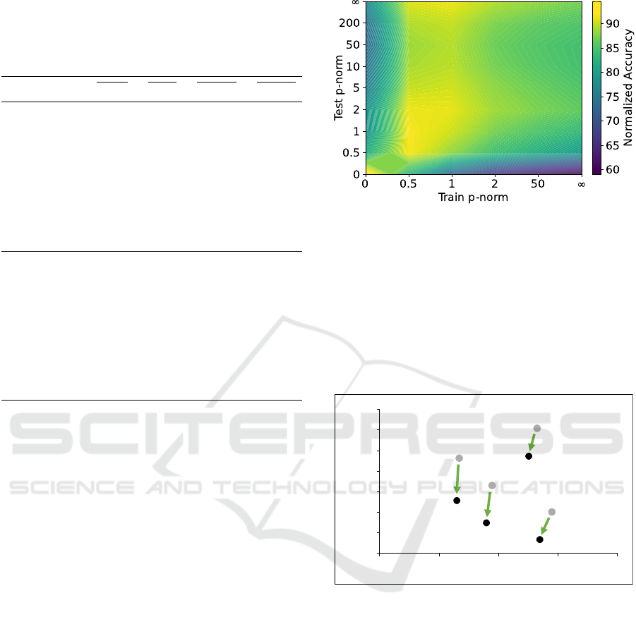
Table 4: The effect of p-norm corruption training types rel-

ative to standard training, averaged across all model archi-

tectures and averaged for the two CIFAR datasets. Largest

average improvement on the dataset for every metric is

marked bold.

Model ∆E

clean

∆mCE ∆mCE

∆mCE

CIFAR

(0.01) +0.3 -4.3 -0.72 -8.96

0.5

(7.5e+4) +1.14 -6.15 -1.73 -10.62

(1) +1.12 -3.69 -1.18 -11.89

∞

(0.02) +1.51 -2.74 -0.33 -10.9

C1 +2.51 -13.04 -4.95 -27.42

C2 +1.79 -12.95 -4.78 -27.86

C3 +1.06 -10.8 -3.45 -25.82

TIN

(0.02) +0.18 -0.8 +0.05 -4.06

0.5

(1.2e+6) -0.11 -0.22 +0.52 -4.39

(2) +0.02 +0.27 +0.82 -2.96

∞

(0.04) +0.77 +0.95 +2.22 -4.47

C1 +1.46 -2.57 -0.46 -14.67

C2 +0.41 -2.81 -0.74 -15.52

C3 -0.14 -2.69 -0.79 -12.13

corruptions of lower p-norms such as L

0.5

and L

are

more suitable for training than corruptions of higher

norms such as L

and L

∞

. The former even achieves

higher robustness against L

∞

-norm corruptions than

∞

-norm training itself.

Table 5 illustrates the effectiveness of the data

augmentation strategies RA, MU, AM and TA. RA

and TA were not evaluated for corruption robustness

in their original publications. The results show that

all methods improve both clean accuracy and robust-

ness. TA achieves the best E

clean

values. It leads to

high robustness values on the CIFAR datasets and es-

pecially on the WRN model. AM is the most effec-

tive method overall in terms of robustness. Our re-

sults show that MU, AM and TA can be improved

by adding combined p-norm corruptions. For the CI-

FAR datasets, additional training with combined p-

norm corruptions only leads to increases in mCE and

mCE

, but not mCE

. On Tiny Imagenet, such ad-

ditional corruptions can, in some combinations, in-

crease mCE

in addition to MU, AM and TA, with-

out any loss of clean accuracy.

All data augmentation strategies still achieve a

signiﬁcant iCE value when not trained with additional

corruptions. The iCE value is much lower for Tiny

Imagenet than for CIFAR.

Figure 4 visualizes E

clean

vs. mCE for selected

model pairs. One of the pairs is additionally trained

with C1 or C2. Models towards the lower left corner

Figure 3: Normalized accuracy when training and testing

on different p-norm corruptions. For each test corruption

(see mCE

in Table 1), the accuracies of all models trained

on p-norm corruptions (without additional data augmenta-

tion strategies) are ﬁrst normalized so that the best model

achieves 100% accuracy. Then the average accuracy is cal-

culated across all model architectures and datasets as well

as across all ε-values of the same p-norm for training and

testing. This visualizes how, on average, training on one

p-norm leads to robustness against all p-norm corruptions.

The prior normalization makes the trained models compa-

rable.

WRN - AM

WRN - AM+C2

WRN - TA

WRN - TA+C1

DN - TA

DN - TA+C1

RNX - TA

RNX - TA+C2

66%

68%

70%

72%

74%

76%

78%

80%

25% 30% 35% 40% 45%

Robust Error [mCE]

Clean Error

Clean vs. Robust Error- Tiny ImageNet

Figure 4: Clean Error vs. mCE plot for selected models

on Tiny Imagenet. The green arrows indicate an improve-

ment of both metrics when the model is trained on p-norm

corruption combinations.

are both more accurate and more robust. The arrows

show how C1 and C2 training can mitigate the trade-

off between accuracy and robustness in these cases.

Figure 6 in the appendix shows how training data

augmentation has an implicit regularizing effect on

the training process, ﬂattening the learning curve.

This effect is evident for the C1 combination, al-

though much less signiﬁcant than for TA. Strong ran-

dom training data augmentation can allow for a longer

training process (Vryniotis, 2021).

VISAPP 2024 - 19th International Conference on Computer Vision Theory and Applications

176

Table 5: The performance of state-of-the-art data augmentation techniques with additional p-norm corruption combinations.

For WRN and RNX, we show those data augmentations that are most effective for at least one metric. The full results are

available on Github.

Model E

clean

mCE mCE

mCE

iCE E

clean

mCE mCE

mCE

iCE E

clean

mCE mCE

mCE

iCE

CIFAR-10 CIFAR-100 TinyImageNet

Standard 5.37 25.38 20.72 28.16 17.2% 23.21 51.33 46.19 53.70 12.4% 37.38 76.46 75.28 53.82 1.4%

RA 4.59 18.25 14.91 21.76 19.0% 21.81 43.87 39.19 49.66 9.6% 35.84 74.53 73.81 52.49 1.4%

MU 4.64 23.39 17.65 29.17 14.7% 22.16 48.96 42.67 53.22 7.7% 35.13 72.81 71.49 50.43 0.6%

MU+C1 5.68 13.89 15.44 7.03 2.1% 23.92 36.96 39.39 26.21 0.5% 36.75 71.40 72.10 38.86 0.2%

MU+C2 5.36 13.77 15.28 6.98 3.5% 23.40 36.88 39.31 25.95 0.6% 35.87 70.79 71.35 38.05 0.5%

MU+C3 4.92 14.65 15.35 8.42 1.9% 22.84 38.22 39.50 28.17 0.2% 35.27 71.20 72.12 42.47 0.4%

AM 4.88 13.14 11.69 13.21 4.6% 23.27 37.90 35.85 37.11 3.6% 36.80 67.03 66.42 49.13 1.9%

AM+C1 5.94 11.32 12.15 7.14 1.1% 25.17 34.86 36.37 27.56 1.0% 38.15 65.19 65.65 40.13 0.2%

AM+C2 5.30 10.58 11.34 6.75 2.1% 24.98 34.50 35.96 27.40 1.2% 38.10 65.02 65.30 40.17 0.2%

AM+C3 5.08 11.34 11.48 8.15 3.6% 24.30 35.32 35.81 29.24 1.0% 37.08 64.12 65.12 43.20 0.5%

TA 4.43 14.25 11.12 17.08 8.4% 20.04 37.85 33.25 42.71 9.0% 34.46 72.61 72.39 72.36 0.7%

TA+C1 5.19 11.94 13.07 6.63 3.3% 22.74 35.27 37.34 25.52 1.2% 33.99 68.97 69.58 36.27 0.2%

TA+C2 5.01 12.88 14.21 6.68 2.3% 22.43 35.32 37.40 25.34 1.4% 34.40 69.91 70.43 36.90 0.5%

TA+C3 4.88 13.36 14.16 7.63 1.8% 21.92 36.36 37.82 26.61 0.5% 34.01 71.48 73.46 40.53 0.4%

WRN

RA 4.56 21.80 18.45 24.02 12.1% 23.25 48.65 44.77 50.96 7.8% 36.89 75.2 73.99 54.05 3.0%

AM+C2 5.53 13.39 14.72 7.13 2.1% 25.40 37.08 39.03 28.01 0.6% 38.48 67.34 67.46 41.22 0.5%

TA 4.13 15.45 11.87 18.68 7.0% 21.70 41.87 37.81 44.32 8.2% 38.25 78.18 77.92 77.88 1.6%

RNX

AM 4.35 14.06 12.13 14.94 9.2% 21.45 38.10 35.31 39.39 4.5% 34.97 67.79 66.09 47.85 1.7%

AM+C2 5.87 11.83 12.87 7.25 2.0% 24.22 33.95 35.60 26.59 0.8% 35.03 65.01 65.52 37.51 0.7%

TA 4.14 15.56 12.55 18.62 10.5% 19.55 37.80 34.28 40.44 6.6% 31.70 75.27 74.98 74.95 2.0%

TA+C2 5.27 14.09 15.86 6.72 0.7% 21.28 35.09 37.52 24.48 1.5% 31.49 71.13 71.99 34.20 0.9%

6 DISCUSSION

Vulnerability to Imperceptible Corruptions. For

the CIFAR datasets in particular, we found iCE val-

ues of well above 10%. Models trained with state-

of-the-art data augmentation methods are still equally

vulnerable to imperceptible random noise. Training

with arbitrary noise outside L

corruptions solves the

problem. We recommend that the set of impercepti-

ble corruptions be further developed as a minimum

requirement for the robustness of vision models, and

that metrics such as iCE be evaluated for this purpose.

Robustness Transfer to Real-World Corruptions

From our experiments we derive insights into improv-

ing real-world robustness by training with p-norm

corruptions:

• Training with single p-norm corruptions generally

leads to mCE improvements only on CIFAR, not

on Tiny ImageNet. The improvements are mainly

attributable to the noise types within mCE. There

is little to negative transfer of robustness against

corruption types outside the pixel-wise noise, rep-

resented by the mCE

metric.

• Training with combinations of p-norm corrup-

tions leads to robustness improvements for the

majority of corruption types outside of pixel-wise

noise

. Thus, mCE

improves even on Tiny Im-

ageNet.

• RA, MU, AM and TA show signiﬁcant robustness

improvements against all real-world corruptions.

• Adding p-norm corruption combinations to RA,

MU, AM and TA gives mixed results. While mCE

often improves, mCE

does so less often. For

Tiny ImageNet, C2 improves mCE

quite effec-

tively on top of all other data augmentation strate-

gies. For CIFAR, mCE

could not be improved

signiﬁcantly beyond AM and TA.

Visit Github for all individual results

Investigating the Corruption Robustness of Image Classiﬁers with Random p-norm Corruptions

177

Robustness Transfer Across p-norms. Given the

limited transferability of robustness between different

types of corruptions known from the literature and the

differences in volume for different p-norm balls (Ta-

ble 6), we expected models trained on one p-norm to

achieve high robustness against that p-norm in par-

ticular. However, we found that training on p-norm

corruptions outside of L

leads to good robustness

against all p-norm corruptions outside of L

. We ﬁnd

that training on L

∞

-norm corruptions performs worse

overall compared to other p-norms. The L

corrup-

tion seems to be a special case that generalizes mainly

to itself. We investigate this behaviour by examin-

ing whether p − norm corruptions overlap in the input

space (see Figure 5 in the appendix).

We ﬁnd that the random L

corruptions are a spe-

cial case in that they almost never share the same in-

put space with an L

-norm ball, and vice versa. In a

weaker form, this is also true for other norms with dis-

similar p like L

∞

-norm and L

. However, when com-

paring corruptions from more similar p-norms like

-norm and L

-norm, we ﬁnd that for most ε val-

ues the corruptions share the same input space. The

observations from Figure 5 explain, from a cover-

age perspective, why corruption robustness seems to

transfer between different p-norms outside of L

. The

∞

-norm is a corner case with the highest p-norm and,

similarly to L

, appears somewhat distinct from L

in Figure 5. Interestingly, our experiments still show

that robustness against high-norm corruptions is most

effectively achieved by training on other p-norm cor-

ruptions.

From the Figures 3 and 5 we conclude that it

makes little difference to train and test on a large vari-

ety of random p-norm corruptions with p > 0. This is

especially true for arbitrarily chosen ε-values like the

set of corruptions for the mCE

-metric. These cor-

ruptions will mostly be sampled in the same region of

the input space and, therefore, be largely redundant.

Promising Data Augmentation Strategies.

From our investigations of robustness transfer across

p-norms we conclude that the C2 strategy is gener-

ally more useful than C1 because it contains only

one p-norm corruption with 0 < p < ∞, whereas

additional such corruptions would be redundant. We

ﬁnd evidence for this assumption in our experimental

results, where on average C2 achieves similar ro-

bustness gains at a lower cost of clean accuracy. In

future work, we would like to investigate whether the

C2 combination can be further improved. First, the

ineffective L

∞

corruption could be reduced in impact.

Second, L

could be replaced by the more effective

0.5

or L

-norm corruptions or by simple Gaussian

noise.

All data augmentation methods MU, RA, AM and

TA improve both corruption robustness and clean ac-

curacy and are therefore highly recommended for all

models and datasets. Therefore, the most relevant

question is whether p-norm corruption training can

be combined with these methods. Our experiments

show a mixed picture: Robustness against noise can

be improved, but robustness against other corruptions

less so. The results vary across datasets, model ar-

chitectures, and base data augmentation methods, as

well as across the different severities of p-norm cor-

ruptions (C1 vs C3). Future progress on this topic

requires precise calibration of the p-norm corruption

combinations and possibly multiple runs of the same

experiment to account for the inherent randomness of

the process and to obtain representative results. In

future work, we aim to improve the p-norm corrup-

tion combinations and apply them for more advanced

training techniques as in (Lim et al., 2021; Erichson

et al., 2022). We believe that this study provides ar-

guments in principle that corruption combinations are

more effective than single noise injections.

7 CONCLUSION

Robustness training and evaluation with random p-

norm corruptions has been little studied in the lit-

erature. We trained and tested three classiﬁcation

models with random p-norm corruptions on three im-

age datasets. We discussed how robustness trans-

fers across p-norms from an empirical and test cov-

erage perspective. The results show that training

data augmentation with L

-norm corruptions is a spe-

ciﬁc corner case. Among all other p-norm corrup-

tions, lower p are more effective for training models.

Combinations of p-norm corruptions are most effec-

tive, which can achieve robustness against corruptions

other than pixel-wise noise. Depending on the setup,

p-norm corruption combinations can improve robust-

ness when applied in sequence with state-of-the-art

data augmentation strategies. We investigated three

different p-norm corruption combinations and, based

on our ﬁndings, made suggestions for further improv-

ing robustness. Our experiments show that several

models, including those trained with state-of-the-art

data augmentation techniques, are negatively affected

by quasi-imperceptible random corruptions. There-

fore, we emphasized the need to evaluate the robust-

ness against such imperceptible corruptions and pro-

posed an appropriate error metric for this purpose. In

the future, we plan to further improve robustness by

more advanced training data augmentation with cor-

ruption combinations.

VISAPP 2024 - 19th International Conference on Computer Vision Theory and Applications

178

REFERENCES

Calaﬁore, G., Dabbene, F., and Tempo, R. (1998). Uni-

form sample generation in l/sub p/balls for probabilis-

tic robustness analysis. In Proceedings of the 37th

IEEE Conference on Decision and Control (Cat. No.

98CH36171), volume 3, pages 3335–3340. IEEE.

Carlini, N., Athalye, A., Papernot, N., Brendel, W., Rauber,

J., Tsipras, D., Goodfellow, I., Madry, A., and Ku-

rakin, A. (2019). On evaluating adversarial robust-

ness. arXiv preprint arXiv:1902.06705.

Carlini, N. and Wagner, D. (2017). Towards evaluating the

robustness of neural networks. In 2017 IEEE Sym-

posium on Security and Privacy (SP), pages 39–57.

IEEE.

Cohen, J. M., Rosenfeld, E., and Kolter, J. Z. (08.02.2019).

Certiﬁed adversarial robustness via randomized

smoothing. International Conference on Machine

Learning (ICML) 2019, page 36.

Croce, F. and Hein, M. (2020). Reliable evaluation of

adversarial robustness with an ensemble of diverse

parameter-free attacks. In International conference on

machine learning, pages 2206–2216. PMLR.

Cubuk, E. D., Zoph, B., Shlens, J., and Le, Q. V. (2020).

Randaugment: Practical automated data augmentation

with a reduced search space. In Proceedings of the

IEEE/CVF conference on computer vision and pattern

recognition workshops, pages 702–703.

Dai, W. and Berleant, D. (2021). Benchmarking robustness

of deep learning classiﬁers using two-factor perturba-

tion. In 2021 IEEE International Conference on Big

Data (Big Data), pages 5085–5094. IEEE.

Dodge, S. and Karam, L. (2017). A study and comparison

of human and deep learning recognition performance

under visual distortions. In 2017 26th international

conference on computer communication and networks

(ICCCN), pages 1–7. IEEE.

Drenkow, N., Sani, N., Shpitser, I., and Unberath, M.

(2021). A systematic review of robustness in deep

learning for computer vision: Mind the gap? arXiv

preprint arXiv:2112.00639.

Erichson, N. B., Lim, S. H., Utrera, F., Xu, W., Cao,

Z., and Mahoney, M. W. (2022). Noisymix: Boost-

ing robustness by combining data augmentations, sta-

bility training, and noise injections. arXiv preprint

arXiv:2202.01263, 1.

Fawzi, A., Fawzi, H., and Fawzi, O. (2018a). Adversar-

ial vulnerability for any classiﬁer. 32nd Conference

on Neural Information Processing Systems (NeurIPS

2018), Montr

eal, Canada.

Fawzi, A., Fawzi, O., and Frossard, P. (2018b). Analysis

of classiﬁers’ robustness to adversarial perturbations.

Machine Learning, 107(3):481–508.

Ford, N., Gilmer, J., Carlini, N., and Cubuk, E. D. (2019).

Adversarial examples are a natural consequence of

test error in noise. Prroceedings of the 36 th Inter-

national Conference on Machine Learning (ICML),

Long Beach, California, PMLR 97, 2019.

Hendrycks, D. and Dietterich, T. (28.03.2019). Bench-

marking neural network robustness to common cor-

ruptions and perturbations. International Conference

on Learning Representations (ICLR) 2019, page 16.

Hendrycks, D., Mu, N., Cubuk, E. D., Zoph, B., Gilmer, J.,

and Lakshminarayanan, B. (05.12.2019). Augmix: A

simple data processing method to improve robustness

and uncertainty. International Conference on Learn-

ing Representations (ICLR) 2020, page 15.

Huang, G., Liu, Z., Van Der Maaten, L., and Weinberger,

K. Q. (2017). Densely connected convolutional net-

works. In Proceedings of the IEEE conference on

computer vision and pattern recognition, pages 4700–

4708.

Huang, X., Kroening, D., Ruan, W., Sharp, J., Sun, Y.,

Thamo, E., Wu, M., and Yi, X. (2020). A sur-

vey of safety and trustworthiness of deep neural net-

works: Veriﬁcation, testing, adversarial attack and de-

fence, and interpretability. Computer Science Review,

37:100270.

Kireev, K., Andriushchenko, M., and Flammarion, N.

(2022). On the effectiveness of adversarial training

against common corruptions. In Uncertainty in Artiﬁ-

cial Intelligence, pages 1012–1021. PMLR.

Krizhevsky, A., Hinton, G., et al. (2009). Learning multiple

layers of features from tiny images. Toronto, Canada.

Krizhevsky, A., Sutskever, I., and Hinton, G. E. (2017). Im-

agenet classiﬁcation with deep convolutional neural

networks. Communications of the ACM, 60(6):84–90.

Le, Y. and Yang, X. (2015). Tiny imagenet visual recogni-

tion challenge. CS 231N, 2015.

Lecuyer, M., Atlidakis, V., Geambasu, R., Hsu, D., and

Jana, S. (2019). Certiﬁed robustness to adversarial ex-

amples with differential privacy. In 2019 IEEE sym-

posium on security and privacy (SP), pages 656–672.

IEEE.

Lim, S. H., Erichson, N. B., Utrera, F., Xu, W., and Ma-

honey, M. W. (2021). Noisy feature mixup. In Inter-

national Conference on Learning Representations.

Lopes, R. G., Yin, D., Poole, B., Gilmer, J., and Cubuk,

E. D. (2019). Improving robustness without sacriﬁc-

ing accuracy with patch gaussian augmentation. arXiv

preprint arXiv:1906.02611.

Loshchilov, I. and Hutter, F. (2016). Sgdr: Stochastic gradi-

ent descent with warm restarts. In International Con-

ference on Learning Representations.

Madry, A., Makelov, A., Schmidt, L., Tsipras, D., and

Vladu, A. (19.06.2017). Towards deep learning mod-

els resistant to adversarial attacks. International Con-

ference on Learning Representations (ICLR) 2018,

page 28.

Mintun, E., Kirillov, A., and Xie, S. (2021). On interaction

between augmentations and corruptions in natural cor-

ruption robustness. Advances in Neural Information

Processing Systems, 34:3571–3583.

uller, S. G. and Hutter, F. (2021). Trivialaugment:

Tuning-free yet state-of-the-art data augmentation. In

Proceedings of the IEEE/CVF international confer-

ence on computer vision, pages 774–782.

Rusak, E., Schott, L., Zimmermann, R. S., Bitterwolf, J.,

Bringmann, O., Bethge, M., and Brendel, W. (2020).

A simple way to make neural networks robust against

Investigating the Corruption Robustness of Image Classiﬁers with Random p-norm Corruptions

179

diverse image corruptions. In European Conference

on Computer Vision (ECCV), pages 53–69. Springer.

Shorten, C. and Khoshgoftaar, T. M. (2019). A survey on

image data augmentation for deep learning. Journal

of big data, 6(1):1–48.

Siedel, G., Vock, S., Morozov, A., and Voß, S. (2022).

Utilizing class separation distance for the evaluation

of corruption robustness of machine learning classi-

ﬁers. The IJCAI-ECAI-22 Workshop on Artiﬁcial In-

telligence Safety (AISafety 2022), July 24-25, 2022,

Vienna, Austria.

Szegedy, C., Zaremba, W., Sutskever, I., Bruna, J., Er-

han, D., Goodfellow, I., and Fergus, R. (2013). In-

triguing properties of neural networks. arXiv preprint

arXiv:1312.6199.

Tsipras, D., Santurkar, S., Engstrom, L., Turner, A., and

Madry, A. (2019). Robustness may be at odds with

accuracy. In International Conference on Learning

Representations.

Vryniotis, V. (2021). How to train state-of-the-art

models using torchvision’s latest primitives.

https://pytorch.org/blog/how-to-train-state-of-the-

art-models-using-torchvision-latest-primitives/,

17.10.2023.

Wang, B., Webb, S., and Rainforth, T. (2021). Statistically

robust neural network classiﬁcation. In Uncertainty in

Artiﬁcial Intelligence, pages 1735–1745. PMLR.

Wang, Z., Bovik, A., Sheikh, H., and Simoncelli, E. (2004).

Image quality assessment: from error visibility to

structural similarity. IEEE Transactions on Image

Processing, 13(4):600–612.

Weng, T.-W., Chen, P.-Y., Nguyen, L. M., Squillante, M. S.,

Boopathy, A., Oseledets, I., and Daniel, L. (2019).

Proven: Verifying robustness of neural networks with

a probabilistic approach. Proceedings of the 36th In-

ternational Conference on Machine Learning, Long

Beach, California, PMLR 97, 2019.

Weng, T.-W., Zhang, H., Chen, P.-Y., Yi, J., Su, D., Gao,

Y., Hsieh, C.-J., and Daniel, L. (2018). Evaluating

the robustness of neural networks: An extreme value

theory approach. Sixth International Conference on

Learning Representations (ICLR), page 18.

Xie, S., Girshick, R., Doll

ar, P., Tu, Z., and He, K. (2017).

Aggregated residual transformations for deep neural

networks. In Proceedings of the IEEE conference on

computer vision and pattern recognition, pages 1492–

1500.

Yang, Y.-Y., Rashtchian, C., Zhang, H., Salakhutdinov, R.,

and Chaudhuri, K. (2020). A closer look at accuracy

vs. robustness. 34th Conference on Neural Informa-

tion Processing Systems (NeurIPS 2020), Vancouver,

Canada.

Yun, S., Han, D., Oh, S. J., Chun, S., Choe, J., and Yoo,

Y. (2019). Cutmix: Regularization strategy to train

strong classiﬁers with localizable features. In Pro-

ceedings of the IEEE/CVF international conference

on computer vision, pages 6023–6032.

Zagoruyko, S. and Komodakis, N. (2016). Wide residual

networks. In British Machine Vision Conference 2016.

British Machine Vision Association.

Zhang, H., Cisse, M., Dauphin, Y. N., and Lopez-Paz, D.

(2018). mixup: Beyond empirical risk minimization.

In International Conference on Learning Representa-

tions.

Zhang, H., Yu, Y., Jiao, J., Xing, E., El Ghaoui, L., and

Jordan, M. (2019). Theoretically principled trade-off

between robustness and accuracy. In International

conference on machine learning, pages 7472–7482.

PMLR.

APPENDIX

Volume of p-norm Balls

Table 6: Volume factors between L

∞

-norm ball and L

norm ball as well as L

-norm ball and L

-norm ball of the

same ε in d-dimensional space.

d p = [∞,2] p = [2,1]

3 1.9 3.1

5 19.7 6.1

10 9037 401.5

20 6 ∗ 10

4 ∗ 10

Sampling Algorithm

We use the following sampling algorithm for norms

0 < p < ∞, which returns a corrupted image I

with

maximum distance ε for a given clean image I of any

dimension d:

1. Generate d independent random scalars x

(G(1/p,1))

1/p

, where G(1/p,1) is a Gamma-

distribution with shape parameter 1/p and scale

parameter 1.

2. Generate I-shaped vector x with components x

∗

, where s

are random signs.

3. Generate scalar r = w

1/d

with w being a random

scalar drawn from a uniform distribution of inter-

val [0,1].

4. Generate n = (

∑

i=1

)

1/p

to norm the ball.

5. Return I

= I + (ε ∗ r ∗ x/n)

The factors r and w allow to adjust the density of

the data points radially within the norm ball. We gen-

erally use a uniform distribution for w except when

we sample imperceptible corruptions (Figure 2).

Volume Overlap of p-norm Balls

In Figure 5 we estimate the overlap of the volumes of

two norm balls with different p and with a dimension-

ality equal to CIFAR-10 (3072). We estimate their

VISAPP 2024 - 19th International Conference on Computer Vision Theory and Applications

180

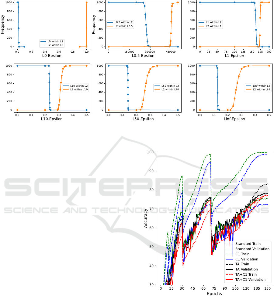
Figure 5: The frequency of 1000 samples drawn from inside a ﬁrst CIFAR-10-dimensional p-norm ball also being part of a

second L

-norm ball of ε = 4 (blue plot), as well as the frequency of 1000 samples drawn from inside the second norm ball

also being part of the ﬁrst norm ball (orange plot).

volumes by uniformly drawing 1000 samples from

inside the norm ball. The ﬁgure shows 6 sub-plots

for different ﬁrst norm balls, where their respective

ε being varied along the x-axis. The blue plots indi-

cate how many samples from this ﬁrst p-norm ball are

also part of a second L

-norm ball with ε = 4. Simi-

larly, the orange plots show how many samples from

the second L

-norm ball are also part of the ﬁrst norm

ball.

There is a large interval of L

− ε-values, where

the samples do not overlap. In a weaker form, this

is also true for other norms far away from p = 2,

like the L

∞

-norm and the L

0.5

-norm. This means

that when comparing L

-norms with e.g. L

-norms,

there is a large range of ε-values, where the two norm

balls cover predominantly different regions of the in-

put space. However, the more similar the p-norms

compared get, like L

with L

, a different result can

be observed. One of the norm balls predominantly

overlaps the other in volume for the widest part of

ε-values. In such a case, the covered input space is

mostly redundant.

Learning Curve Effect

When added to a standard or TA training procedure,

the training curve of the C1 model is more ﬂat (Figure

6. TA itself shows a very strong ﬂattening effect on

the learning curve and requires visibly more epochs

to converge.

Figure 6: Training and validation learning curves of vari-

ous models show the slight regularizing effect of p-norm

corruptions in the C1 combination on the training process.

Investigating the Corruption Robustness of Image Classiﬁers with Random p-norm Corruptions

181