
Two Nonlocal Variational Models for Retinex Image Decomposition
Frank W. Hammond
1 a
, Catalina Sbert
2 b
and Joan Duran
2 c
1
Higher Polytechnic School, University of the Balearic Islands, Spain
2
Department of Mathematics and Computer Science & IAC3, University of the Balearic Islands,
Cra. de Valldemossa, km. 7.5, E-07122 Palma, Illes Balears, Spain
Keywords:
Retinex Theory, Illumination, Reflectance, Image Decomposition, Low-Light Enhancement, Variational
Method, Total Variation, Nonlocal Regularization.
Abstract:
Retinex theory assumes that an image can be decomposed into illumination and reflectance components. In this
work, we introduce two variational models to solve the ill-posed inverse problem of estimating illumination
and reflectance from a given observation. Nonlocal regularization exploiting image self-similarities is used
to estimate the reflectance, since it is assumed to contain fine details and texture. The difference between the
proposed models comes from the selected prior for the illumination. Specifically, Tychonoff regularization,
which promots smooth solutions, and the total variation, which favours piecewise constant solutions, are
independently proposed. A comprehensive theoretical analysis of the resulting functionals is presented within
appropriate functional spaces, complemented by an experimental validation for thorough examination.
1 INTRODUCTION
The Retinex theory (Land and McCann, 1971) aims
to explain and simulate how the human visual system
perceives color independently of global illumination
changes. Accordingly, an image can be decomposed
into luminance and reflectance components.
Many implementations of Retinex have been pro-
posed in the literature. Based on the center/surround
alternative algorithm (Land, 1986), Jobson et al. (Job-
son et al., 1996; Jobson et al., 1997) introduced a
method that filters the input image with Gaussian ker-
nels, taking the low-frequency result as the illumi-
nation and the residual image as the reflectance. In
(Horn, 1974; Morel et al., 2010), the Poisson equa-
tion is used to perform the decomposition.
Decomposing and image into illumination and
reflectance is mathematically ill-posed, thus prior
knowledge on the solution needs to be assumed. The
regularization theory assumes that the image which
is to be reconstructed is sufficiently smooth. In the
variational framework, this is formulated through the
minimization of functionals that induce a high energy
when the priors are not fulfilled.
Kimmel et al. (Kimmel et al., 2001) pioneered a
a
https://orcid.org/0009-0005-6890-0202
b
https://orcid.org/0000-0003-1219-4474
c
https://orcid.org/0000-0003-0043-1663
variational model to estimate the illumination, which
is assumed to be spatially smooth, in a multiscale set-
ting. The reflectance is not considered and needs to be
computed in post-processing. Guo et al. (Guo et al.,
2017) infer the illumination as the minimizer of a sim-
ple energy functional that incorporates the total vari-
ation (TV) seminorm as regularization term (Rudin
et al., 1992). The reflectance is obtained by pixelwise
divison between the input image and the estimated il-
lumination. However, this approach tends to amplify
the noise, especially in dark regions. To overcome this
issue, the use of denoising techniques becomes essen-
tial. Ng and Wang (Ng and Wang, 2011) estimate
illumination and reflectance simultaneously, penaliz-
ing gradient oscillations in the illumination through
L
2
norm and using TV for the reflectance, which is
thus assumed to be piecewise constant.
Many other variational methods perform the de-
composition in the logarithmic domain. In this set-
ting, Fu et al. (Fu et al., 2016) proposed a weighted
gradient-based variational model to avoid issues when
either the reflectance or the illumination is small.
Recently, an increasing number of deep learning
methods with different architectures have been pro-
posed (Chen et al., 2018; Wu et al., 2022). However,
these approaches are less flexible and interpretable
than model-based methods, and the training and test-
ing of the networks require high computational costs.
Hammond, F., Sbert, C. and Duran, J.
Two Nonlocal Variational Models for Retinex Image Decomposition.
DOI: 10.5220/0012396800003660
Paper published under CC license (CC BY-NC-ND 4.0)
In Proceedings of the 19th International Joint Conference on Computer Vision, Imaging and Computer Graphics Theory and Applications (VISIGRAPP 2024) - Volume 3: VISAPP, pages
551-558
ISBN: 978-989-758-679-8; ISSN: 2184-4321
Proceedings Copyright © 2024 by SCITEPRESS – Science and Technology Publications, Lda.
551

In this paper, we propose two variational models
to simulatenously estimate the illumination and re-
flectante components of an image. In both cases, non-
local regularization exploiting image self-similarities
is used to estimate the reflectance, since it is assumed
to contain fine details and texture. For the illumina-
tion, Tychonoff regularization, favouring smooth so-
lutions, and TV, favouring piecewise constant solu-
tions, are independently proposed. A comprehensive
study of the existence and uniqueness of minimizers
in suitable functional spaces is provided.
The rest of the paper is organized as follows. In
Section 2, we present the nonlocal spaces and display
some tools from nonlocal vector calculus. Section 3
is devoted to the proposed models, where we prove
the existence and uniqueness of minimizer and intro-
duce the saddle-point formulations that will be used to
compute the solutions through the first-order primal-
dual algorithm by Chambolle and Pock (Chambolle
and Pock, 2011). Section 4 evaluates the performance
of the proposed methods and compares them with
some state-of-the-art techniques. Finally, conclusions
are drawn in Section 5.
2 NONLOCAL THEORY
TV assumes that images consist of connected smooth
regions (objects) surrounded by sharp contours. Ac-
cordingly, it is optimal to reduce noise and reconstruct
the main geometry, but it fails to preserve fine details.
On the contrary, nonlocal regularization (Gilboa and
Osher, 2009; Duran et al., 2014) allows any point to
interact directly with any other point in the domain.
The resemblance between them is usually evaluated
by comparing a patch around each point. Thus, the
underlying assumption is that images are self-similar,
thereby preserving fine details and texture.
In this section, we introduce weighted L
p
spaces,
for which nonlocal regularization is well defined, and
formalize a systematic and coherent framework for
nonlocal operators. Let Ω be a finite-measure sub-
set of R
n
, with n ≥2, and w: Ω →[0,+∞) a bounded
measurable function that is nonzero a.e. in Ω.
2.1 Weighted L
p
Spaces
Let p ∈ [1,+∞]. We define the weighted L
p
space as
L
p
w
(Ω) =
f : Ω → R :
Z
Ω
(|f |
p
w)dx < +∞
,
which is endowed with the norm ∥f ∥
p,w
= ∥f w
1/p
∥
p
.
Note that, in order ∥·∥
p,w
to be a norm, w must be
nonzero a.e. in Ω, otherwise it will be a seminorm.
It is easy to show that L
p
w
(Ω) is a Banach space
containing L
p
(Ω), for p ∈ [1,+∞]. We are interested
in L
2
w
(Ω), which is a Hilbert space equipped with the
scalar product
⟨
f ,g
⟩
2,w
=
⟨
f
√
w,g
√
w
⟩
2
=
R
Ω
f gw dx.
Definition 2.1. We define the difference function of
u ∈ L
p
(Ω) as
b
u(x,y) = u(y) −u(x).
Note that ∥
b
u∥
p
≤2|Ω|
1/p
∥u∥
p
, where the norm on
the left is the L
p
(Ω×Ω)-norm and the one on the right
is the L
p
(Ω)-norm. Therefore,
b
u ∈ L
p
(Ω ×Ω).
Proposition 2.1. Let {u
n
}
n∈N
be a sequence in L
2
(Ω)
converging weakly to u in L
2
(Ω). Then, {
b
u
n
}
n∈N
con-
verges weakly to
b
u in L
2
w
(Ω).
Proof. Since L
2
w
(Ω ×Ω) is a Hilbert space, we can
identify f
∗
with some f ∈ L
2
w
(Ω × Ω) such that
f
∗
(x) =
⟨
f ,x
⟩
. We have
⟨
f ,
b
u
n
⟩
2,w
=
Z
Ω
Z
Ω
(u
n
(y) −u
n
(x)) f (x,y)w(x, y)dxdy.
Let us define the functions F(x) =
R
Ω
f (x, y)w(x,y)dy
and G(y) =
R
Ω
f (x, y)w(x,y)dx. Then,
(F(x))
2
≤
|
Ω
|
M
Z
Ω
f (x, y)
2
w(x,y)dy,
where M is an upper bound for w, so that
R
Ω
(F(x))
2
dx ≤ M|Ω| · ∥f ∥
2
2,w
< +∞. Thus, F ∈
L
2
(Ω). Similarly, it can be proved that G ∈ L
2
(Ω). It
follows that f
∗
(
b
u
n
) →
⟨
u,G
⟩
2
−
⟨
u,F
⟩
2
= f
∗
(
b
u).
Corollary 2.2. Let {u
n
}
n∈N
be a sequence in L
2
(Ω)
converging weakly to u in L
2
(Ω). Then,
liminf
n
∥
b
u
n
∥
2,w
≥ ∥
b
u∥
2,w
Proof. It follows from previous result and weak lower
semicontinuity of norms in a Banach spaces.
2.2 Basic Nonlocal Vector Calculus
The notion of directional derivative extends to the
nonlocal case as ∂
y
u(x) =
b
u(x,y)
p
w(x,y). The non-
local gradient is then defined as the vector of nonlocal
derivatives, i.e., ∇
w
u(x,y) = ∂
y
u(x).
The nonlocal divergence is defined to satisfy the
adjoint relation
⟨
∇
w
u,v
⟩
2,Ω×Ω
=
⟨
u,−div
w
(v)
⟩
2,Ω
. A
sufficient condition for this is defining
div
w
(v)(x) =
Z
Ω
v(y, x)
p
w(y, x) −v(x, y)
p
w(x,y)dy.
3 PROPOSED MODELS
Let us assume that the observed image S defined on Ω
is the product of the illumination L ∈ (0,+∞) and the
VISAPP 2024 - 19th International Conference on Computer Vision Theory and Applications
552

reflectance R ∈ (0,1). By transforming S = R ·L into
the logarithmic domain, we get
l = s + r, (1)
where l = log(L), s = log(S) and r = −log(R). Based
on (1), we introduce two nonlocal variational models
to estimate l and r simultaneously, using nonlocal reg-
ularization for the reflectance, assumed to contain fine
details and texture, and testing Tychonoff and TV for
the luminance, assumed to be smooth.
To find a global optimal solution to the proposed
minimization problems, we use the first-order primal-
dual algorithm introduced in (Chambolle and Pock,
2011). Therefore, we rewrite each problem in a
saddle-point formulation by introducing dual vari-
ables. The algorithm consists of alternating a gra-
dient ascent in the dual variable, a gradient descent
in the primal variable, and an over-relaxation for
convergence purposes. The gradient steps are given
in terms of proximity operators, which are defined
for any proper convex function ϕ as prox
τ
ϕ(x) =
argmin
y
ϕ(y) +
1
2τ
∥x −y∥
2
2
. For all details on convex
and functional analysis omitted in this section, we re-
fer to (Br
´
ezis, 2011; Chambolle and Pock, 2016).
3.1 Nonlocal and Tychonoff Terms
We propose to estimate r and l as the minimizers of
E
1
(r, l) = ∥
b
r∥
2
2,w
+
α
2
∥|∇l|∥
2
2
+
β
2
∥l −r −s∥
2
2
+
γ
2
∥l∥
2
2
(2)
where α, β, γ > 0 are trade-off parameters. The last
term is added for purely technical reasons and has no
actual practical significance.
Theorem 3.1. Let Λ = L
2
(Ω)×W
1,2
(Ω) be the space
of admissible functions and s ∈L
2
(Ω). There exists a
unique (r
∗
,l
∗
) ∈ Λ s.t. E
1
(r
∗
,l
∗
) = inf
(r,l)∈Λ
E
1
(r, l).
Proof. Existence. We follow the direct method and a
proof similar to that in (Ng and Wang, 2011).
It is easy to see that E
1
is proper and bounded be-
low, thus b = inf
(r,l)∈Λ
E
1
(r, l) < ∞. Let {(r
n
,l
n
)}⊆Λ
be such that E
1
(r
n
,l
n
) → b.
Since E
1
(r
n
,l
n
) is uniformly bounded, so are
R
Ω
|∇l
n
|
2
and ∥l
n
∥
2
, implying that {l
n
} is uniformly
bounded in W
1,2
(Ω). By the Rellich-Kondrachov the-
orem, there exists l
∗
∈ L
2
(Ω) such that l
n
→ l
∗
in
L
2
(Ω), and, up to a subsequence, l
n
⇀ l
∗
in W
1,2
(Ω)
due to the space being reflexive.
Furthermore, {r
n
} is uniformly bounded in L
2
(Ω)
as ∥r
n
∥
2
≤ ∥l
n
−r
n
−s∥
2
+ ∥s∥
2
+ ∥l
n
∥
2
. Thus, there
exists r
∗
∈L
2
(Ω) s.t., up to a subsequence, r
n
⇀ r
∗
in
L
2
(Ω). By Proposition 2.1,
b
r
n
⇀
b
r
∗
in L
2
w
(Ω ×Ω).
Finally, due to the weak lower semicontinuity of
the norms, b = lim inf
n
E
1
(r
n
,l
n
) ≥ E
1
(r
∗
,l
∗
) ≥ b,
from which we deduce E
1
(r
∗
,l
∗
) = b.
Uniqueness. It is a direct consequence of E
1
being
strictly convex.
3.1.1 Saddle-Point Optimization
Let Λ
′
= L
2
(Ω ×Ω) ×
L
2
(Ω)
n
and K : Λ → Λ
′
be
the linear operator K(r,l) = (∇
w
r, ∇l). We also con-
sider G : Λ → [0,+∞] and F : Λ
′
→ [0,+∞], respec-
tively defined as G(r,l) =
β
2
∥r −l −s∥
2
2
+
γ
2
∥l∥
2
2
and
F(a, b) = ∥a∥
2
2
+
α
2
∥
|
b
|
∥
2
2
.
The minimization of (2) can be rewritten in a
saddle-point formulation as
min
(r,l)∈Λ
sup
(a,b)∈Λ
′
⟨
(a,b),K(r,l)
⟩
−F
∗
(a,b) + G(r,l),
where F
∗
denotes the convex conjugate of F.
In practice, the initial values of a sequence gen-
erated by an iterative algorithm may have errors due
to arbitrary initialization, which can accumulate and
lead to undesired results in the final image. To miti-
gate this, an additional constraint is introduced. Since
l = s + r, with r ≥ 0, then l ≥ s. Therefore, it makes
sense to impose both r ≥ 0 and l ≥ s.
Finally, the luminance l and the reflectance r
are computed through the following Chambolle-Pock
primal-dual iterates, that is, initialize over-relaxiation
variables ˜r
0
= r
0
= 0,
˜
l
0
= l
0
= s, and update the dual
variables as follows:
a
n+1
b
n+1
= prox
σF
∗
a
n
+ σ∇
w
(˜r
n
)
b
n
+ σ∇
˜
l
n
Then, update the primal variables, impose the con-
straints r ≥ 0, l ≥ s and update the over-relaxation
variables.
r
n+1/2
l
n+1/2
= prox
τG
r
n
+ τdiv
w
(a
n+1
)
l
n
+ τdiv(b
n+1
)
r
n+1
= max(r
n+1/2
,0), l
n+1
= max(l
n+1/2
,s)
˜r
n+1
= 2r
r+1
−r
n
,
˜
l
n+1
= 2l
n+1
−l
n
The proximity operators involved are
prox
τG
a
b
=
(βτ+γτ+1)a+βτb−βτ(γτ+1)s
βγτ
2
+2βτ+γτ+1
βτa+(βτ+1)b+βτs
βγτ
2
+2βτ+γτ+1
!
prox
σF
∗
a
b
=
a
1+σ/2
b
1+σ/α
!
3.2 Nonlocal and TV Terms
We take s ∈ L
2
(Ω) and α, β,γ positive numbers,
and consider the functional E
2
over Λ = L
2
(Ω) ×
Two Nonlocal Variational Models for Retinex Image Decomposition
553

Building Lamp Bookcase
Horses Papiervert
Figure 1: Dataset used for the experiments.
BV(Ω) ∩L
2
(Ω)
:
E
2
(r, l) = ∥
b
r∥
2
2,w
+ αTV(l) +
β
2
∥l −r −s∥
2
2
+
γ
2
∥l∥
2
2
.
(3)
Theorem 3.2. There exists a unique (r
∗
,l
∗
) ∈ Λ such
that
E
2
(r
∗
,l
∗
) = inf
r,l
E
2
(r, l)
Proof. Existence. This proof is very similar to that
of Theorem 3.1. E
2
is clearly a proper functional,
and thus we can consider a minimizing sequence
E
2
(r
n
,l
n
) → b = inf E
2
. Again, each of the additive
terms of E
2
(r
n
,l
n
) will be uniformly bounded.
From Holder inequality it follows that
∥
l
n
∥
1
≤
|
Ω
|
1/2
∥
l
n
∥
2
is uniformly bounded.
Therefore, {TV(l
n
)}
n∈N
and {
∥
l
n
∥
1
}
n∈N
are uni-
formly bounded, whence {l
n
}
n∈N
is bounded in
BV(Ω). Therefore, there exists some l
∗
∈ BV(Ω)
such that, up to a subsequence,
l
n
L
1
(Ω)
→ l
∗
and l
n
L
2
(Ω)
⇀ l
∗
∈ L
2
(Ω).
Because of the lower semicontinuity of norms in
BV(Ω) and L
2
(Ω),
liminf
n
αTV(l
n
) +
γ
2
∥
l
n
∥
2
2
≥ αTV(l
∗
) +
γ
2
∥
l
∗
∥
2
2
This, as in 3.1, implies that E
2
(r
∗
,l
∗
) = b.
Uniqueness. Again, a direct consequence of the
functional being strictly convex.
3.2.1 Saddle-Point Optimization
The same primal-dual algorithm as in the previous
section is used. The problem obtained is
min
r,l
T (K(r,l)) + G(r,l),
with K(r,l) = (∇
w
r, ∇l), T (a,b) =
∥
a
∥
2
2
+ α
∥
|b|
∥
1
and G(r,l) =
β
2
∥
l −r −s
∥
2
2
+
γ
2
∥
l
∥
2
2
is the same as in
the Tychonoff functional. The algorithm used is very
similar, the only difference being that the dual vari-
ables are updated via the proximity operator of T
∗
:
a
n+1
b
n+1
= prox
σT
∗
a
n
+ σ∇
w
(˜r
n
)
b
n
+ σ∇
˜
l
n
The proximity operator is computed as follows:
prox
σT
∗
a
b
=
a
1+σ/2
b
max(1,
|
b
|
/α)
!
3.3 Proposed Weights
For the nonlocal regularization term in both mod-
els, we need to select an appropriate weight func-
tion w : Ω ×Ω → [0,+∞). We propose to use bilat-
eral weights that consider both the spatial closeness
between points and the similarity in the input image
S : Ω → R
C
. This similarity is computed by consid-
ering a whole patch around each point and using the
Euclidean distance across the color channels:
d
a
(S(x),S (y)) =
Z
Ω
G
a
(z)
|
S(x + z) −S(y + z)
|
2
dz,
where |·| denotes the Euclidian norm in R
C
and G
a
is
a Gaussian kernel of standard deviation a ≥ 0.
The weights are defined as
w(x,y) =
1
Γ(x)
exp
−
|x −y|
2
h
2
spt
−
d
a
(S(x),S (y))
h
2
sim
!
,
(4)
where h
spt
,h
sim
> 0 are filtering parameters that con-
trol how fast the weights decay with increasing spa-
tial distance or dissimilarity between patches, respec-
tively, and Γ(x) is the normalization factor
Γ(x) =
Z
Ω
exp
−
|x −y|
2
h
2
spt
−
d
a
(S(x),S (y))
h
2
sim
!
dy.
Note that 0 < w(x,y) ≤ 1 and
R
Ω
w(x,y)dy = 1, but
the normalization factor breaks down the symmetry
of w. In the end, the average made between very sim-
ilar regions preserves the integrity of the image but
reduces its small oscillations, which contain noise.
For computational purposes, the nonlocal regular-
ization is limited to interact only between points at a
certain distance. Accordingly, the weight distribution
is in general sparse since a few nonzero values are
considered. In this setting, let N (x) denote a neigh-
bourhood around each x ∈Ω. Then, w(x,y) is defined
as in (4) if y ∈ N (x), and zero otherwise. The nor-
malization factor is finally given by
Γ(x) =
Z
N (x)
exp
−
|x −y|
2
h
2
spt
−
d
a
(L(x),L(y))
h
2
sim
!
dy.
VISAPP 2024 - 19th International Conference on Computer Vision Theory and Applications
554
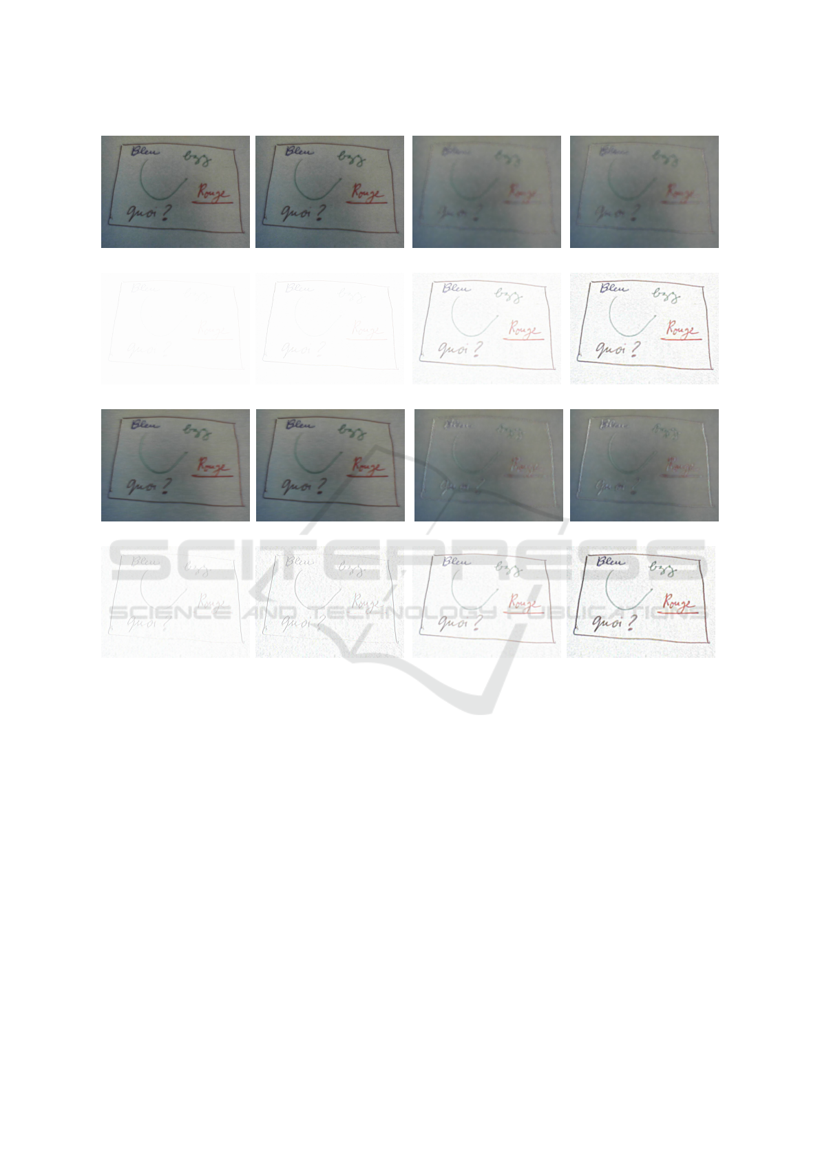
α = 0.1,β = 0.1 α = 0.1,β = 5 α = 5,β = 0.1 α = 5,β = 5
Figure 2: Visual impact of the trade-off parameters α and β in the proposed models for the Papiervert image. The estimated
illumination maps are displayed in the first and third rows for (2) and (3), respectively. The corresponding reflectance compo-
nents are displayed in the second and fourth rows for (2) and (3), respectively. Larger values of the regularization parameter
α provide smoother illumination components, while the geometry and colors remain in the reflectance maps. We observe that
the shadows due to lighting conditions are retained in the illumination components. Furthermore, the difference between the
two proposed models is evident in the estimated illumination maps. The results from (2) tend to be isotropically smooth due
to the use of a Tychonoff prior, while the results from (3) are piecewise constant, as expected from the TV.
In practice, the weight of the reference point is
set to the maximum of the weights in the neihbour-
hood, w(x,x) = max{w(x, y) : y ∈ N (x)}. This set-
ting avoids the excessive weighting of the reference
point. Furthermore, G
a
is not considered as it is only
necessary when the size of N (x) is large.
4 ANALYSIS AND EXPERIMENTS
In this section, we analyze the performance of the
proposed method for illumination and reflectance de-
composition. Figure 1 displays the images we used
in all experiments: Building (Petro et al., 2014),
Lamp (Guo et al., 2017), Bookcase (Wei et al., 2018),
Horses (Petro et al., 2014) and Papiervert (Morel
et al., 2010).
For our variational methods, we fix the follow-
ing parameters throughout the experimental section:
γ = 10
−5
, h
spt
= 1.25, h
sim
= 2.5 and the number of
iterations is set to 2000. We revert the logarithmic
transformation by applying the exponential function
to the outputs of the primal-dual algorithm.
In Figure 2 we display the decomposition results
Two Nonlocal Variational Models for Retinex Image Decomposition
555
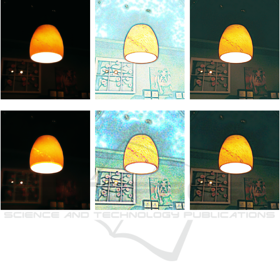
Illumination Reflectance Enhanced image
Figure 3: Resulting decomposition (α = 1, β = 5) of Lamp by the proposed Tychonoff (2) (first row) and TV (3) (second
row) models, and the respective enhanced images after applying a gamma correction with parameter 0.4 to the illumination
component. We observe that the geometry, texture, color information, and noise are retained in the reflectance maps. Further-
more, the enhanced image by a simple gamma correction is able to discount the effect of the ilumination in the scene. We also
observe that the ilumination map produced by Tychonoff is isotropically smooth while that of TV is piecewise constant.
for different α and β combinations in both models on
Papiervert. Values were chosen taking into account
that the nonlocal regularization term has a coefficient
of 1 in both models. Thus, the smaller the values α,β
are in relation to 1, the more importance is given to
nonlocal regularization. In both models, bigger val-
ues for α tend to yield smoother results for illumina-
tion, which was to be expected since we are imposing
that |∇l| be small in the functional. Smaller values
for α tend to yield illumination approximations that
are very close to the original image, and reflectance
approximations which are very close to R = 1. Big-
ger values for β tend to produce better results, since
this parameter corresponds to our fidelity term. How-
ever, values too big (>> 20, as experience indicates),
tend to produce decompositions with the illumination
approximation too close to the original image. We
observe that the shadows due to lighting conditions
are retained in the illumination components. Further-
more, the difference between the two proposed mod-
els is evident in the estimated illumination maps. The
results from (2) tend to be isotropically smooth due
to the use of a Tychonoff prior, while the results from
(3) are piecewise constant, as expected from the TV.
Experience shows that best results are often ob-
tained for values of α and β smaller than 20, bigger
than 1 and β ≥ α. We propose α = 1, β = 5 as default
parameters in both models.
In Figure 3, we show the decomposition of Lamp
for our default combination α = 1 and β = 5. A
gamma correction of 0.4 is applied to illumination (al-
though the corrected version is not displayed) before
computing the resulting image.
In Figure 4, we compare the performance of our
method with state-of-the-art techniques Multiscale
Retinex (MSR) (Jobson et al., 1997), Kimmel et al.
VISAPP 2024 - 19th International Conference on Computer Vision Theory and Applications
556
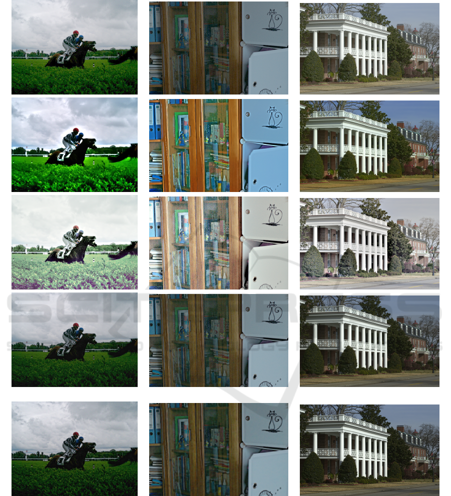
α = 1, β = 10, Correction 0.5 α = 2, β = 10, Correction 0.35 α = 1, β = 5, Correction 0.6
α = 1, β = 10, Correction 0.5 α = 1, β = 1, Correction 0.35 α = 1, β = 5, Correction 0.6
Figure 4: Comparison between state-of-the-art techniques for low-light image enhancement and our models combined with a
gamma correction to the illumination component. Each row contains the results by Kimmel et al., LIME, MSR, our Tychonoff
model (2), and our TV model (3). Compared to our proposals, the method by Kimmel et al. produces similar results in terms of
illumination, but is more sensitive to noise, LIME produces oversaturated colors, while MSR is not robust to noise and exhibits
color issues. Our methods provide a good compromise between discounting the illumination, avoiding the amplification of
noise, and preserving color and geometry. Note also that the results by Tychonoff are slightly more blurred than those of TV,
as seen in the clouds and grass of Horses and on trees on Building.
Two Nonlocal Variational Models for Retinex Image Decomposition
557

(Kimmel et al., 2001) and LIME (Guo et al., 2017)
on Horses, Bookcase and Building. The most suitable
parameters for all methods have been chosen based
on visual evaluation. We observe that neither MSR
nor the method proposed by Kimmel et al. are robust
to noise, LIME oversaturates color and MSR yields
greyish images. In contrast, both our methods cor-
rectly enhance illumination, respect color and are rel-
atively robust to noise. The Tychonoff model pre-
serves color slightly better than TV, but contrasts are
clearer in the latter.
5 CONCLUSION
In this paper, we proposed two variational models
to simultaneously estimate the luminance and re-
flectance components from an observed image. Non-
local regularization has been employed as a prior for
the reflectance to help preserve colors and texture. Ty-
chonoff and TV regularizations have been tested for
the illumination component. We utilized this decom-
position for low-light image enhancement.
In future work, it may be interesting to explore
more sophisticated methods to enhance illumination
and experiment with different mechanisms to reduce
noise in our estimation of reflectance.
ACKNOWLEDGEMENTS
This work is part of the MaLiSat project TED2021-
132644B-I00, funded by MCIN/AEI/10.13039/
501100011033/ and by the European Union
NextGenerationEU/PRTR, and also of the Mo-
LaLIP project PID2021-125711OB-I00, financed by
MCIN/AEI/10.13039/501100011033/FEDER, EU.
In memoriam Frank G. Hammond Figueroa.
REFERENCES
Br
´
ezis, H. (2011). Functional analysis, Sobolev spaces and
partial differential equations, volume 2. Springer.
Chambolle, A. and Pock, T. (2011). A first-order primal-
dual algorithm for convex problems with applications
to imaging. Journal of mathematical imaging and vi-
sion, 40:120–145.
Chambolle, A. and Pock, T. (2016). An introduction to
continuous optimization for imaging. Acta Numerica,
25:161–319.
Chen, W., Wenjing, W., Wenhan, Y., and Jiaying, L. (2018).
Deep retinex decomposition for low-light enhance-
ment. In British Machine Vision Conference.
Duran, J., Buades, A., Coll, B., and Sbert, C. (2014). A
nonlocal variational model for pansharpening image
fusion. SIAM Journal on Imaging Sciences, 7(2):761–
796.
Fu, X., Zeng, D., Huang, Y., Zhang, X., and Ding, X.
(2016). A weighted variational model for simultane-
ous reflectance and illumination estimation. CVPR,
pages 2782–2790.
Gilboa, G. and Osher, S. (2009). Nonlocal operators with
applications to image processing. Multiscale Model-
ing & Simulation, 7(3):1005–1028.
Guo, X., Yu, L., and Ling, H. (2017). Lime: Low-light
image enhancement via illumination map estimation.
IEEE Transactions on Image Processing, 26(2):982–
993.
Horn, B. K. (1974). Determining lightness from an image.
Computer Graphics and Image Processing, 3(4):277–
299.
Jobson, D., Rahman, Z., and Woodell, G. (1996). Properties
and performance of a center/surround retinex. TIP,
6(3):451–462.
Jobson, D., Rahman, Z., and Woodell, G. (1997). A multi-
scale retinex for bridging the gap between color im-
ages and the human observation of scenes. IEEE
Transactions on Image Processing, 6(7):965–976.
Kimmel, R., Elad, M., Shaked, D., Keshet, R., and Sobel,
I. (2001). A variational framework for retinex. Int. J.
Comput. Vis., 52(1):7–23.
Land, E. (1986). An alternative technique for the compu-
tation of the designator in the retinex theory of color
vision. In Proc. of the National Academy of Science,
volume 83 of 10, pages 3078–3080.
Land, E. H. and McCann, J. J. (1971). Lightness and retinex
theory. Josa, 61(1):1–11.
Morel, J. M., Petro, A. B., and Sbert, C. (2010). A pde
formalization of retinex theory. IEEE Transactions on
Image Processing, 19(11):2825–2837.
Ng, M. K. and Wang, W. (2011). A total variation model
for retinex. SIAM Journal on Imaging Sciences,
4(1):345–365.
Petro, A. B., Sbert, C., and Morel, J.-M. (2014). Multi-
scale Retinex. Image Processing On Line, pages 71–
88. https://doi.org/10.5201/ipol.2014.107.
Rudin, L. I., Osher, S., and Fatemi, E. (1992). Nonlinear to-
tal variation based noise removal algorithms. Physica
D: nonlinear phenomena, 60(1-4):259–268.
Wei, C., Wang, W., Yang, W., and Liu, J. (2018). Deep
retinex decomposition for low-light enhancement.
BMVC.
Wu, W., Weng, J., Zhang, P., Wang, X., Yang, W., and Jiang,
J. (2022). Uretinex-net: Retinex-based deep unfold-
ing network for low-light image enhancement. In Pro-
ceedings of the IEEE/CVF conference on computer vi-
sion and pattern recognition, pages 5901–5910.
VISAPP 2024 - 19th International Conference on Computer Vision Theory and Applications
558
