An Optimised Ensemble Approach for Multivariate Multi-Step Forecasts

Using the Example of Flood Levels

Michel Spils

and Sven Tomforde

Department of Computer Science, University of Kiel, Kiel, Germany

Keywords:

Machine Learning, Time-Series Forecasting, Ensemble Deep Learning, Flood Forecasting.

Abstract:

Deep Learning methods have become increasingly popular for time-series forecasting in recent years. One

common way of improving time-series forecasts is to use ensembles. By combining forecasts of different

models, for example calculating the mean forecast, it is possible to get an ensemble that performs better than

each single member. This paper suggests a method of aggregating ensemble forecasts using another neural

network.The focus is on multivariate multi-step ahead forecasting. Experiments are done on 5 water levels at

small to medium-sized rivers and show improvements on naive ensembles and single neural networks.

1 INTRODUCTION

Flood and disaster protection are typically sovereign

tasks of local authorities and include not only coastal

regions but also areas of inﬂuence of ﬂowing wa-

ters of different sizes. For example, the State Of-

ﬁce for the Environment in Schleswig-Holstein, Ger-

many’s northernmost federal state, operates 182 gaug-

ing stations close to in-land rivers where water levels

and ﬂow behaviour are determined and forecasts are

made. On the basis of these forecasts, disaster control

measures are taken if necessary. One challenging as-

pect of forecasting water levels is the lack of training

data. It is not possible to simply simulate the environ-

ment, the only way to gather more data for a gauging

station is to wait.

The application scenario requires very reliable

forecasts of water levels, as protective measures are

taken on this basis. At the same time, this places

special demands on forecasting methods because, on

the one hand, conditions are not static due to climate

change and changes in topology and, on the other

hand, the focus is on extreme events. Thus, a devi-

ation of a few percent in normal behaviour is abso-

lutely uncritical, whereas this is essential in the case

of ﬂoods. Hence, the overall goal is to investigate a

self-adaptive and self-learning forecast system with a

continuous assessment of uncertainty, reliability and

impact of the determined forecasts.

https://orcid.org/0000-0002-6431-6085

https://orcid.org/0000-0002-5825-8915

In this paper, we present a novel approach to gen-

erate and use ensembles for water level prediction.

Based on previous work on the forecast quality of

single predictors, we investigate to what extent an

ensemble of optimised models improves the forecast

quality. This is combined with an approach to op-

timise the weighting within the ensemble in order to

achieve a further gain in prediction quality and robust-

ness. We analyse the impact inﬂuence factors of the

observed behaviour and provide the considered data

of the experiments.

The remainder of this paper is organised as fol-

lows: Section 2 describes the current state-of-the-art

from a technical and an application point of view.

Section 3 introduces our approach for an ensemble-

based forecasting of ﬂood levels. Afterwards, Sec-

tion 4 introduces the underlying data and metrics, fol-

lowed by a description of base models and execution

time. The analysis of the experimental results as well

as the insights and ﬁndings are discussed in Section 5.

Finally, Section 6 summarises the paper and describes

future work.

2 RELATED WORK

In the ﬁrst subsection 2.1 we give a short overview of

ﬂood forecasting using Machine learning in general,

in subsection 2.2 we focus on different ways of using

ensembles for forecasting.

388

Spils, M. and Tomforde, S.

An Optimised Ensemble Approach for Multivariate Multi-Step Forecasts Using the Example of Flood Levels.

DOI: 10.5220/0012396000003636

Paper published under CC license (CC BY-NC-ND 4.0)

In Proceedings of the 16th International Conference on Agents and Artiﬁcial Intelligence (ICAART 2024) - Volume 2, pages 388-396

ISBN: 978-989-758-680-4; ISSN: 2184-433X

2.1 Flood Forecasting

In (Kratzert et al., 2021) Long Short-Term Memory

networks (LSTMs) are used to simulate ﬂow rates

based on meteorological observations. They ﬁnd that

it is possible to (pre-)train a single model to predict

ﬂow rates at multiple basins. The authors of (Hu

et al., 2018) study the performance of LSTMs com-

pared to standard neural networks for ﬂood forecast-

ing and ﬁnd that they perform signiﬁcantly better. In

(Kao et al., 2020) the authors explore LSTM based

Encoder-Decoder architectures for multi-step-ahead

ﬂood forecasting.

In (Grundmann et al., 2020) the use of precipi-

tation forecast ensembles for ﬂood forecasting is in-

vestigated. The German Weather Service provides an

ensemble with 20 members of high-resolution pre-

cipitation forecasts, which is useful for rare events

with strong rainfall that are not represented in the

main forecast. (Morgenstern et al., 2022) enrich their

LSTM input with statistical information such as area

maximum, minimum and standard deviation of pre-

cipitation intensity. (Wee et al., 2021) and (Mosavi

et al., 2018) give a general overview of water level and

ﬂood forecasting using machine learning. Most re-

search on ﬂood forecasting focuses on large rivers and

on either very short forecast horizon, up to six hours

ahead or on daily forecast. We attempt to forecast

water levels with a forecast horizon up to 48 hours at

small to medium sized rivers with a catchment area of

up to 600km

2.2 Ensemble-Based Forecasting

In (Sommer et al., 2016), a ﬁrst study has been pre-

sented that aims at re-weighting the ensemble based

on current conditions using an evolutionary reinforce-

ment learning paradigm (XCSF/eXtended Classiﬁer

System for Function approximation). Moreira-Matias

et al. (Moreira-Matias et al., 2013) use the error

of their base models on a sliding window to di-

rectly weigh their ensemble. In a more recent ap-

proach (Choi and Lee, 2018) change the ensemble

weights at each step based. This is again based on

the base models error on a sliding window, but is also

parametrized by a learning rate λ and a discount factor

γ which weights more recent errors higher. (Cerqueira

et al., 2017) train a second model for each base model

that predicts the expected error, this error is then used

to weight the ensemble. Later they extended this ap-

proach to also consider model diversity (Cerqueira

et al., 2018). In (Saadallah and Morik, 2021) a Deep

Deterministic Policy Gradient (DDPG) model is used

to combine univariate single horizon forecasts. The

RL uses a sliding window of past forecasts as state

and the rank of the ensemble model compared with

the base models as the reward. One approach explic-

itly designed for multi-horizon forecasting approxi-

mates optimal weights by calculating a weighted lin-

ear regression on either the training data or a slid-

ing window of past data (Galicia et al., 2019). In

(Gheyas and Smith, 2011) a set of base learners is

trained on pairwise disjoint subsets of available fea-

tures. The output of the base learners is used as input

to another model, after undergoing feature selection.

In (Casanova and Ahrens, 2009) the authors evalu-

ate equal weighting, simple skill-based weighting and

Bayesian model averaging for weather forecasting.

Most existing approaches do not take the current

input into account and instead rely on recent or his-

toric performance. We supply the input to the base

models to our weighting approach so that very recent

changes in the situation such as a unexpected rainfall

can be considered when weighting the ensemble.

3 PROPOSED ENSEMBLE

WEIGHTING APPROACH

In this section we present our approach to combine

forecasting ensembles. The basic idea of our ap-

proach is to directly weight the ensemble forecast us-

ing a neural network, instead of the usual approach of

using the ensemble forecast as input to another neu-

ral network or alternative machine learning algorithm.

First, a set of arbitrary base learners is trained. This

has the advantage that each model is trained indepen-

dently, which allows us to take advantage of hyperpa-

rameter optimization, unlike dependent frameworks

like AdaBoost.

(x,y)

Model 1

Dense

Layers

Model N...

Concat

Normalize

(e.g. softmax)

Matmul

Figure 1: Ensemble weighting architecture.

The ensemble model is a neural network with two

paths. One path with an arbitrary but constant number

of base learners and the second path with a small num-

An Optimised Ensemble Approach for Multivariate Multi-Step Forecasts Using the Example of Flood Levels

389

ber of layers to predict the weighting matrix. Cur-

rently, a number of dense layers is used to predict the

optimal weighting, but the exact architecture is arbi-

trary. To calculate the ﬁnal output the model does an

element-wise multiplication of the concatenated out-

puts of the base models and the weight matrix.

Figure 1 shows this architecture.

The ensemble model has the task of optimizing

the weighting for n base models and the current input

data x. The ensemble model calculates a matrix of

weights w which is normalized so that w

i, j

≥ 0 and

∑

i=1

i, j

= 1 for each forecast step j ∈ {1, . . . , h}.

This guarantees that the forecast of the ensemble

model is bounded by the minimum and maximum of

the base forecasts. Whether this is a positive or a neg-

ative constraint depends on the quality and diversity

of the base models.

This can be done in different ways, the optimal

normalization function likely depends on the distribu-

tion of model quality. We tested linear normalization,

which is deﬁned as:

′

w − min(w)

∑

i=1

− min(w))

(1)

And the softmax function:

′

exp(w)

∑

i=1

(exp(w

))

(2)

To calculate the ﬁnal output the ensemble model

does an element-wise multiplication of the concate-

nated outputs of the base models and the weight ma-

trix. The meta-learner is trained on the same data as

the base models. During the training process of the

meta-learner, the base models are frozen. It is not

technically necessary to implement this with the base

models as part of the meta-learner and it may be more

computationally efﬁcient to cache the forecasts made

by the base models.

4 DATASETS AND BASE MODELS

In this section, we ﬁrst introduce our datasets and

evaluation metrics. We then describe our base models

or learners and how long the training took.

4.1 Datasets

The 5 datasets used in this paper represent the dif-

ferent water levels that we attempt to forecasts and

contain publicly available data. They all contain sen-

sor and radar data and values derived from the sensor

data. The target value of each dataset is the water

level of a river in Schleswig-Holstein, Germany. Ad-

ditionally, they contain precipitation forecasts that are

synthesized by shifting the calculated precipitation 48

hours into the past. In a production environment, this

synthetic forecast would be replaced by the ICON D2

forecast (Reinert et al., 2020). The input data for each

gauge is a subset of the nearest available sensor sta-

tions measuring air temperature, air pressure, air hu-

midity, soil moisture, evaporation, and up- and down-

stream water levels. The aggregate data and all used

source code will be made available on request. The

goal is to predict the water levels for the next 48 hours

from the past water levels and other sensor data.

Figure 2 shows a map of the 458.6km

catchment

of the water level Foehrden-Barl at the river Stoer.

The green dot represents the location of the target wa-

ter level, the black dots represent the location of up-

stream water levels and the blue dot the location of

the nearest air temperature and air humidity sensor.

The three marked areas represent subcatchments for

which precipitation was calculated. For the Foehrden-

Barl dataset soil moisture and air pressure data was

used, but the sensor stations are outside the area on

the map.

Figure 2: Map of the catchment Foehrden-Barl.

All features are sampled hourly, but some derived

values like soil moisture are upsampled from daily

calculations. For training all data was standardized

to a mean of zero and a standard deviation of one.

Table 1: The ﬁve datasets used in the experiments.

Dataset Features Length

Foehrden-Barl 13 61360

Hollingstedt 9 71542

Halstenbek 5 83816

Poetrau 5 77699

Willenscharen 10 77434

ICAART 2024 - 16th International Conference on Agents and Artiﬁcial Intelligence

390

4.2 Evaluation Metrics

We track several metrics for our experiments, but for

the sake of brevity and readability we only include

the Weighted Average Percentage error (WAPE) and

the Nash–Sutcliffe model efﬁciency coefﬁcient (NSE)

in this paper. The WAPE of each forecast horizon is

deﬁned as

WAPE =

∑

t=1

− ˆy

∑

t=1

(3)

with T the number of observations, y

the true value

and ˆy

the predicted value.

The NSE is a standard metric for hydrological

models. A perfect model would result in a NSE of

1, a model that just predicts the mean observed value

in a NSE of 0.

NSE = 1 −

∑

t=1

− ˆy

)

∑

t=1

− y)

(4)

with y being the mean observed value.

4.3 Base Learner

For each dataset, we trained 24 neural networks as en-

semble members. All models were trained on the ﬁrst

70% of each dataset, with the following 15% parts

as validation and test set. To reduce overﬁtting train-

ing was stopped whenever the validation loss did not

reduce for three epochs. On average this happened af-

ter 23 epochs. Table 2 shows the (hyper-)parameters

of all base models. We exclusively used LSTM net-

works, because preliminary testing showed that they

outperform other architectures in both performance

and training speed for our datasets. On average the

MAE of models using for example a Transformer ar-

chitecture was 25% higher and models using the Aut-

oformer architecture ((Wu et al., 2022)) were 50%

higher, while taking 3-4 longer to train.

4.4 Execution Time

Training neural networks can be very expensive, so it

is important not to ignore the computational cost of

new approaches. All training was done on a single

Nvidia A100 GPU with 80GB memory. Training the

base models took on average 55s, with a minimum of

12s and a maximum of 93s. Training the ensemble

models took on average 40s, with a minimum of 10s

and a maximum of 129s. The cost of our approach of

training a neural network to combine an ensemble of

models is in the same order of magnitude as the the

cost of training a single neural network.

Table 2: Base learner parameters.

Parameter Value

Input window 144 hours

Output window 48 hours

Learning rate 0.001

Loss function MSE

Optimizer Adam

Batch size 4096

Max Epochs 100

Dropout 0.25

LSTM Layers [1,2]

LSTM Units [64,128,256]

Hidden layers [1,2]

Hidden layer units [128,256]

5 EXPERIMENTS AND RESULTS

This section contains descriptions of our experiments

and their results.

5.1 Experiment 1: Static Model Set,

Hyperparameter Optimization

For this experiment, we did a hyperparameter opti-

mization for the ensemble model with a ﬁxed set of

base models. We used Tree-structured Parzen Esti-

mator (TPE) for sampling and trained 100 models,

minimizing the validation loss. Table 3 shows the hy-

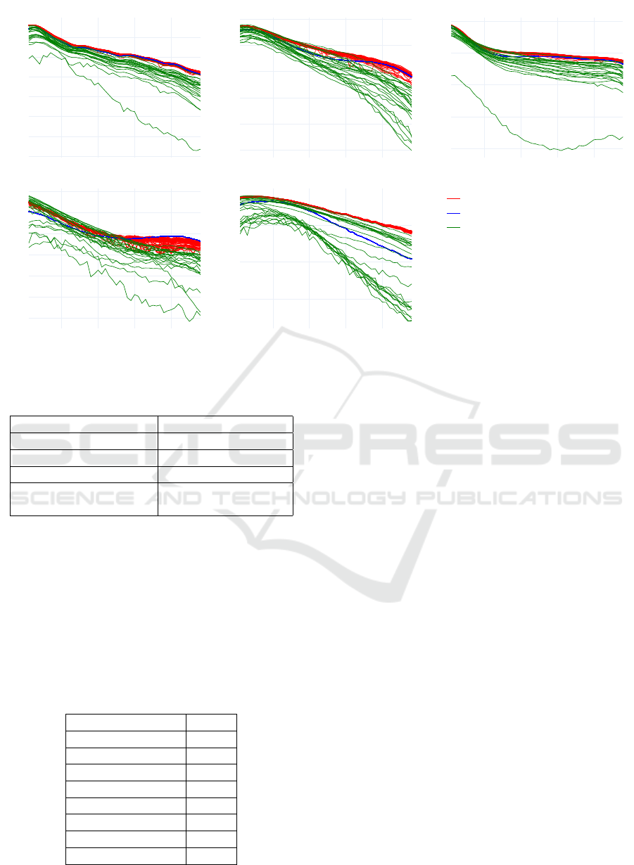
perparameter constraints. In Figure 3 the NSE val-

ues of each ensemble model, the base model and the

mean forecast of the base model set is displayed. The

ensemble model has a higher thus better NSE than

the base models with nearly all tester hyperparame-

ters, except at the water level Poetrau, where the base

models perform better with small forecast horizons.

Figure 4 shows the results of the hyperparameter-

optimization. The linear/minmax normalization re-

sults in a lower validation loss for all datasets ex-

cept Poetrau. The optimal found hyperparameters dif-

fer between the datasets. There is no clear optimal

amount of hidden layers and hidden units. There is a

trend towards a low learning rate being better, but for

Foehrden-Barl a larger learning rate leads to better re-

sults. The range of the model quality of the ensemble

model is much smaller than the range of quality for

base models.

An Optimised Ensemble Approach for Multivariate Multi-Step Forecasts Using the Example of Flood Levels

391

10 20 30 40

0.86

0.88

0.9

0.92

0.94

0.96

0.98

10 20 30 40

0.75

0.8

0.85

0.9

0.95

10 20 30 40

0.6

0.7

0.8

0.9

10 20 30 40

0.7

0.75

0.8

0.85

0.9

0.95

10 20 30 40

0.85

0.9

0.95

Ensemble model

Ensemble mean

Base models

Hollingstedt validation Willenscharen validation Halstenbek validation

Poetrau validation Foehrdenbarl validation

Forecast Horizon (hours)

NSE

Figure 3: NSE for ensemble models with ﬁxed base model set, mean of these sets and base models.

Table 3: Constraints hyperparameter optimization.

Parameter Value range

Learning rate 0.00001 ≤ 0.01

Hidden layers 0 ≤ n ≤ 2

Hidden layer units 32 ≤ n ≤ 512

Normalization function Linear normalization

or Softmax

5.2 Experiment 2: Random Model Set,

Static Hyperparameters

For this experiment, we trained 100 ensemble models

with a random set of 10 base models each. The hy-

perparameters for our ensemble models can be seen

in Table 4. Gradient Clipping was used for improved

learning.

Table 4: Ensemble model ﬁxed parameters.

Parameter Value

Learning rate 0.002

Loss function MSE

Optimizer Adam

Batch size 2048

Max Epochs 100

Dropout 0.25

Hidden layers 2

Hidden layer units 512

Figure 5 shows the WAPE for all ﬁve datasets at

different forecast horizons. The mean WAPE of the

ensemble models is lower than the mean WAPE of

the base models for all datasets and forecasts horizons

and lower than the mean WAPE of the naive model

ensembles for all datasets and horizons except Poet-

rau with 48h. In most cases, the mean WAPE of the

ensemble models is better or comparable to the best

base model.

5.3 Discussion

Both experiments show that our approach outper-

forms both the base models and the naive ensemble

for most datasets and forecast horizons. The ﬁrst ex-

periment shows that there is no clear best normaliza-

tion function. This combined with the comparatively

bad results for dataset Poetrau in the second experi-

ment is a sign that some hyperparameter optimization

may be necessary to reliably outperform naive ensem-

bles for some datasets. LSTM-Ensembles strongly

outperform single LSTM models.

While there are several studies that investigate

ﬂood forecasting with neural networks (Tripathy and

Mishra, 2023), it is not easy to directly compare these

studies. There are two main reasons for this. First

the used data. Authors tend to study catchments and

rivers geographically close to them. Since rivers can

behave very different depending on for example size

and mean catchment slope many metrics are not di-

rectly comparable. A low MAE at a large stream is

ICAART 2024 - 16th International Conference on Agents and Artiﬁcial Intelligence

392

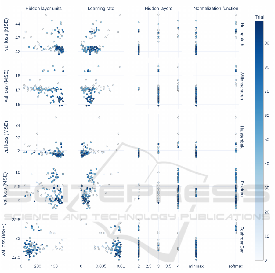
Figure 4: Validation loss for different datasets and hyperparameters.

much easier to achieve than in a small river. Addi-

tionally, the used data differs. Some only learn on

events with heavy rainfall, other on the whole dataset.

Many papers simply use precipitation and discharge

stations to predict the future discharge, others include

evaporation data and precipitation forecasts. Some

make daily forecasts, other hourly. The second obsta-

cle when comparing studies is the variety of metrics

that are used to evaluate model quality, there is no

single metric that is used in every paper. One study

found that Spatio-Temporal Attention LSTM models

(STA-LSTM) worked best for discharge forecasting

(Ding et al., 2020). They reported coefﬁcient of deter-

mination (R

) values of 0.92, 0.75 and 0.84 for three

different catchments. These values interestingly are

the mean R

of lead times 1h to 6h. Using this metric

our ensembles with a static model set have an average

of value of:

• Hollingstedt: 0.990

• Willenscharen: 0.988

• Halstenbek: 0.967

• Poetrau: 0.965

• Foehrdenbarl: 0.986

Another study, which investigated a 329km

large

basin in Texas, found that synced sequence input and

output (SISO) LSTM is the best performing LSTM ar-

chitecture for ﬂood prediction (Li et al., 2020). They

An Optimised Ensemble Approach for Multivariate Multi-Step Forecasts Using the Example of Flood Levels

393

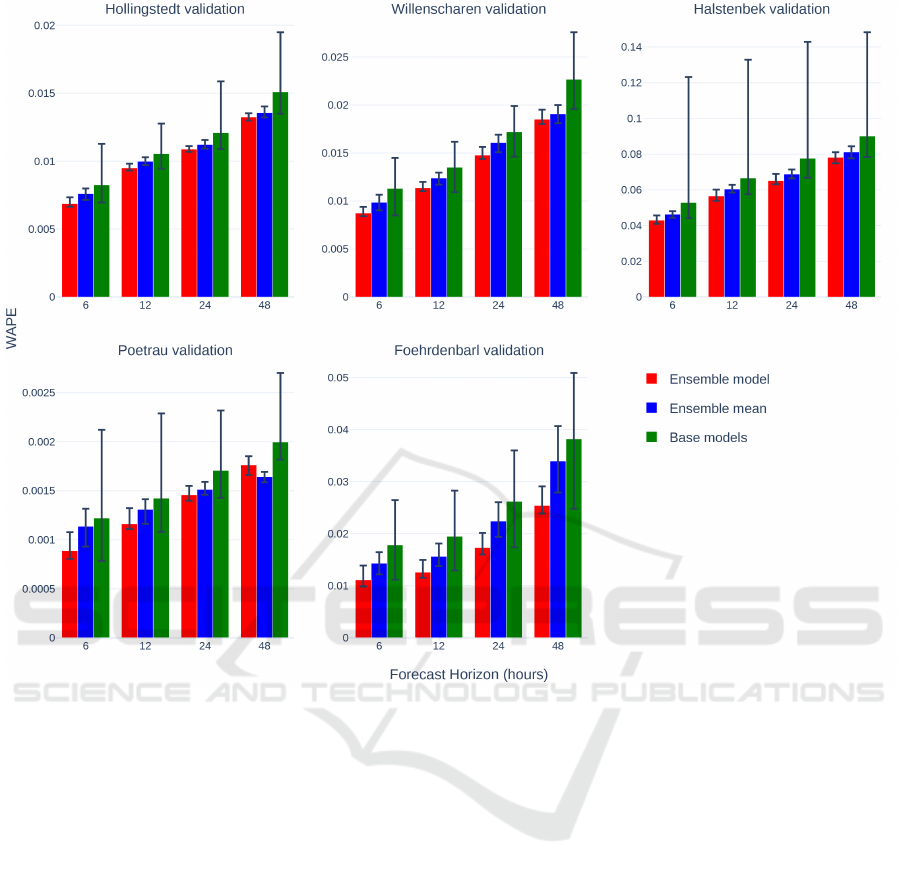
Figure 5: Mean, minimum and maximum WAPE for ensemble models with random sets of base models, mean of these sets

and base models.

use rainfall and discharge gauges sampled at 15 min-

utes as input and report an NSE of .943, but the lead

time of their forecast regrettably stays unclear. One

study, which also used precipitation forecasts, found

that context-aware attention LSTM (CA-LSTM) out-

perform regular LSTM, but are outperformed by fully

connected neural networks (FCN) for lead times up to

2h. The used data was taken from 40 ﬂood events at a

single river. They report an average root-mean-square

error (RMSE) of 59.95 over up to 6h lead time, a met-

ric that we did not track.

6 CONCLUSION AND FUTURE

WORK

This section recaps our results and suggests some di-

rections for further research.

6.1 Conclusion

In this paper, we developed a new method of com-

bining multivariate multi-step forecast ensembles and

tested our method on water level data. Our method

outperformed naive ensembles and base learners on

most datasets and forecast horizons, but we have not

compared our approach to other state-of-the-art en-

semble approaches, because very few investigate mul-

tivariate multi-step forecasts. The ﬁrst experiment

showed that the choice of hyperparameters, especially

the normalization function, has some inﬂuence on

the ensemble model quality but the variance is much

lower than for the base models. The second exper-

iment showed that our approach works random base

model sets and usually works without any hyperpa-

rameter optimization. Training the ensemble model

is very fast, taking about as long as training a single

base model with an LSTM architecture. This, com-

bined with the fact that the base models are trained

independently from the ensemble model, allowing us

ICAART 2024 - 16th International Conference on Agents and Artiﬁcial Intelligence

394

to very efﬁciently build ensemble models that outper-

form naive ensembles and can offset bad-performing

base models. Since modern machine learning ap-

proaches often undergo a hyperparameter optimiza-

tion resulting in many decent, but not optimal model

we can use our approach to improve from those mod-

els a nearly no cost.

6.2 Future Work

Currently, both the weighting method and the model

sets are fairly naive. In future work we plan to inves-

tigate more sophisticated methods. The base models

currently share the same architecture and training data

and only differ in hyperparameters. Modern ensemble

approaches often consider model diversity when se-

lecting base models. Doing the same in our approach

could result in a fairly large improvement since the

ensemble model can only forecasts correctly if the

ground truth is between minimum and maximum base

forecast. We also have not yet investigated the inﬂu-

ence of the size of our ensembles. Larger ensembles

could potentially perform even better but may need

different normalization functions and weighting ar-

chitectures. Another direction we would like to in-

vestigate are adaptive model sets. Using the perfor-

mance of base models on different benchmark data

as additional input would allow us to change the set

of base models. This would be useful if there is a

drift in our data. With long-term drifts being common

in hydrological data we intend to also extend our ap-

proach towards training and retraining models at run

time instead of just weighting a static model set, thus

adapting to changed environments.

ACKNOWLEDGEMENTS

The used data is mostly publicly available from DWD

(German Meteorological Service) and the LfU-SH

(Landesamt f

ur Umwelt Schleswig-Holstein), kindly

aggregated by the LfU-SH. This research was sup-

ported by the Federal State of Schleswig-Holstein in

the context of the “KI-F

orderrichtlinie” under grant

220 22 05 (project KI-WaVo).

REFERENCES

Casanova, S. and Ahrens, B. (2009). Oq. Monthly Weather

Review, 137(11):3811–3822.

Cerqueira, V., Torgo, L., Pinto, F., and Soares, C.

(2017). Arbitrated ensemble for time series forecast-

ing. In Machine Learning and Knowledge Discovery

in Databases, pages 478–494. Springer International

Publishing.

Cerqueira, V., Torgo, L., Pinto, F., and Soares, C. (2018).

Arbitrage of forecasting experts. Machine Learning,

108(6):913–944.

Choi, J. Y. and Lee, B. (2018). Combining LSTM network

ensemble via adaptive weighting for improved time

series forecasting. Mathematical Problems in Engi-

neering, 2018:1–8.

Ding, Y., Zhu, Y., Feng, J., Zhang, P., and Cheng, Z. (2020).

Interpretable spatio-temporal attention lstm model for

ﬂood forecasting. Neurocomputing, 403:348–359.

Galicia, A., Talavera-Llames, R., Troncoso, A., Koprinska,

I., and Mart

ınez-

Alvarez, F. (2019). Multi-step fore-

casting for big data time series based on ensemble

learning. Knowledge-Based Systems, 163:830–841.

Gheyas, I. A. and Smith, L. S. (2011). A novel neural net-

work ensemble architecture for time series forecast-

ing. Neurocomputing, 74(18):3855–3864.

Grundmann, J., Six, A., and Philipp, A. (2020). Ensem-

ble hydrological forecasting for ﬂood warning in small

catchments in saxony, germany.

Hu, C., Wu, Q., Li, H., Jian, S., Li, N., and Lou, Z. (2018).

Deep learning with a long short-term memory net-

works approach for rainfall-runoff simulation. Water,

10(11):1543.

Kao, I.-F., Zhou, Y., Chang, L.-C., and Chang, F.-J. (2020).

Exploring a long short-term memory based encoder-

decoder framework for multi-step-ahead ﬂood fore-

casting. Journal of Hydrology, 583:124631.

Kratzert, F., Gauch, M., Nearing, G., Hochreiter, S., and

Klotz, D. (2021). Niederschlags-abﬂuss-modellierung

mit long short-term memory (lstm).

Osterreichische

Wasser-und Abfallwirtschaft, 73(7-8):270–280.

Li, W., Kiaghadi, A., and Dawson, C. (2020). Explor-

ing the best sequence lstm modeling architecture for

ﬂood prediction. Neural Computing and Applications,

33(11):5571–5580.

Moreira-Matias, L., Gama, J., Ferreira, M., Mendes-

Moreira, J., and Damas, L. (2013). Predicting

taxi–passenger demand using streaming data. IEEE

Transactions on Intelligent Transportation Systems,

14(3):1393–1402.

Morgenstern, T., Grundmann, J., and Sch

utze, N. (2022).

Flood forecasting with LSTM networks: Enhancing

the input data with statistical precipitation informa-

tion.

Mosavi, A., Ozturk, P., and Chau, K.-w. (2018). Flood pre-

diction using machine learning models: Literature re-

view. Water, 10(11):1536.

Reinert, D., Prill, F., Frank, H., Denhard, M., Baldauf, M.,

Schraff, C., Gebhardt, C., Marsigli, C., and Z

angl,

G. (2020). Dwd database reference for the global

and regional icon and icon-eps forecasting system.

DWD 2023Available online: https://www. dwd.

de/DWD/forschung/nwv/fepub/icon database main.

pdf (accessed on 27 January 2023).

Saadallah, A. and Morik, K. (2021). Online ensemble ag-

gregation using deep reinforcement learning for time

series forecasting. In 2021 IEEE 8

International

An Optimised Ensemble Approach for Multivariate Multi-Step Forecasts Using the Example of Flood Levels

395

Conference on Data Science and Advanced Analytics

(DSAA). IEEE.

Sommer, M., Stein, A., and H

ahner, J. (2016). Local ensem-

ble weighting in the context of time series forecasting

using xcsf. In 2016 IEEE Symposium Series on Com-

putational Intelligence (SSCI), pages 1–8. IEEE.

Tripathy, K. P. and Mishra, A. K. (2023). Deep learning in

hydrology and water resources disciplines: concepts,

methods, applications, and research directions. Jour-

nal of Hydrology, page 130458.

Wee, W. J., Zaini, N. B., Ahmed, A. N., and El-Shaﬁe, A.

(2021). A review of models for water level forecasting

based on machine learning. Earth Science Informat-

ics, 14(4):1707–1728.

Wu, H., Xu, J., Wang, J., and Long, M. (2022). Autoformer:

Decomposition transformers with auto-correlation for

long-term series forecasting.

ICAART 2024 - 16th International Conference on Agents and Artiﬁcial Intelligence

396