Parameter-Free Connectivity for Point Clouds

Diana Marin

, Stefan Ohrhallinger

and Michael Wimmer

Institute of Visual Computing & Human-Centered Technology, TU Wien, Austria

Keywords:

Proximity Graphs, Point Clouds, Connectivity.

Abstract:

Determining connectivity in unstructured point clouds is a long-standing problem that has still not been ad-

dressed satisfactorily. In this paper, we analyze an alternative to the often-used k-nearest neighborhood (kNN)

graph - the Spheres of Inﬂuence Graph (SIG). We show that the edges that are neighboring each vertex are

spatially bounded, which allows for fast computation of SIG. Our approach shows a better encoding of the

ground truth connectivity compared to the kNN for a wide range of k, and additionally, it is parameter-free.

Our result for this fundamental task offers potential for many applications relying on kNN, e.g., parameter-free

normal estimation, and consequently, surface reconstruction, motion planning, simulations, and many more.

1 INTRODUCTION

In recent times, point clouds have gained popular-

ity as a data representation, owing to advancements

in scanning technology. However, the initial state

of disorganized points necessitates further process-

ing to reconstruct the original surface’s connectiv-

ity from which they were sampled. This connec-

tivity allows for the estimation of surface properties

such as neighborhoods or normals. Various meth-

ods are available for estimating the intrinsic proper-

ties of point clouds, but they often rely on selecting

the appropriate parameters tailored to the speciﬁc data

type. For instance, this includes determining neigh-

borhood connectivity using the user-speciﬁed ‘k’ in

k-nearest neighbor (kNN) calculations. Additionally,

point cloud sampling can be non-uniform due to the

acquisition method or tainted by artifacts like noise

and outliers. These conditions make the process of

parameter selection for scanned data a challenging

and time-consuming endeavor.

Extracting connectivity from point clouds is a

signiﬁcant research challenge, not only due to its

essential role as a ﬁrst step in surface reconstruction

but also because it forms the foundational input for

graph-based learning tasks involving point clouds.

Regarding surface reconstruction, connectivity

graphs serve as the fundamental structure on which

triangles are constructed, and as a computation base

for normals, which are sometimes required as part

of the reconstruction process. For learning-based

https://orcid.org/0000-0002-8812-9719

https://orcid.org/0000-0002-2526-7700

https://orcid.org/0000-0002-9370-2663

tasks, establishing a method for connecting the input

points that closely aligns with the original surface is

imperative, since the creation of an actual surface is

not necessary.

We propose a fast computation of the spheres-of-

inﬂuence graph (SIG) and we analyze its properties

as a proximity graph. This graph recovers the original

connectivity of the surface better than the widely

used kNN graph, as it can be seen in Figure 1, while

dropping the need for users to search for a suitable

parameter that typically varies depending on the input

and its local properties. Our method achieves the

best results on various models with different features.

Hence, our method offers a good scaffolding for

further processing of point clouds, such as normal

estimation, surface reconstruction, or graph convo-

lutional neural networks. We show that our method

not only encodes the original connectivity better than

kNN but, as an application, provides a good base for

normal estimation, while remaining parameter-free.

We present the following contributions:

• We introduce an effective method for construct-

ing the spheres-of-inﬂuence graph, proving novel

spatial constraints for this parameter-free graph.

• Our method is evaluated against ground truth

meshes, demonstrating superior connectivity rep-

resentation with a reduced space requirement

when compared to traditional kNN graphs.

• As an application, we offer an analysis of nor-

mal computation on point clouds, highlighting our

method’s ability to deliver competitive results.

Marin, D., Ohrhallinger, S. and Wimmer, M.

Parameter-Free Connectivity for Point Clouds.

DOI: 10.5220/0012394900003660

Paper published under CC license (CC BY-NC-ND 4.0)

In Proceedings of the 19th International Joint Conference on Computer Vision, Imaging and Computer Graphics Theory and Applications (VISIGRAPP 2024) - Volume 1: GRAPP, HUCAPP

and IVAPP, pages 92-102

ISBN: 978-989-758-679-8; ISSN: 2184-4321

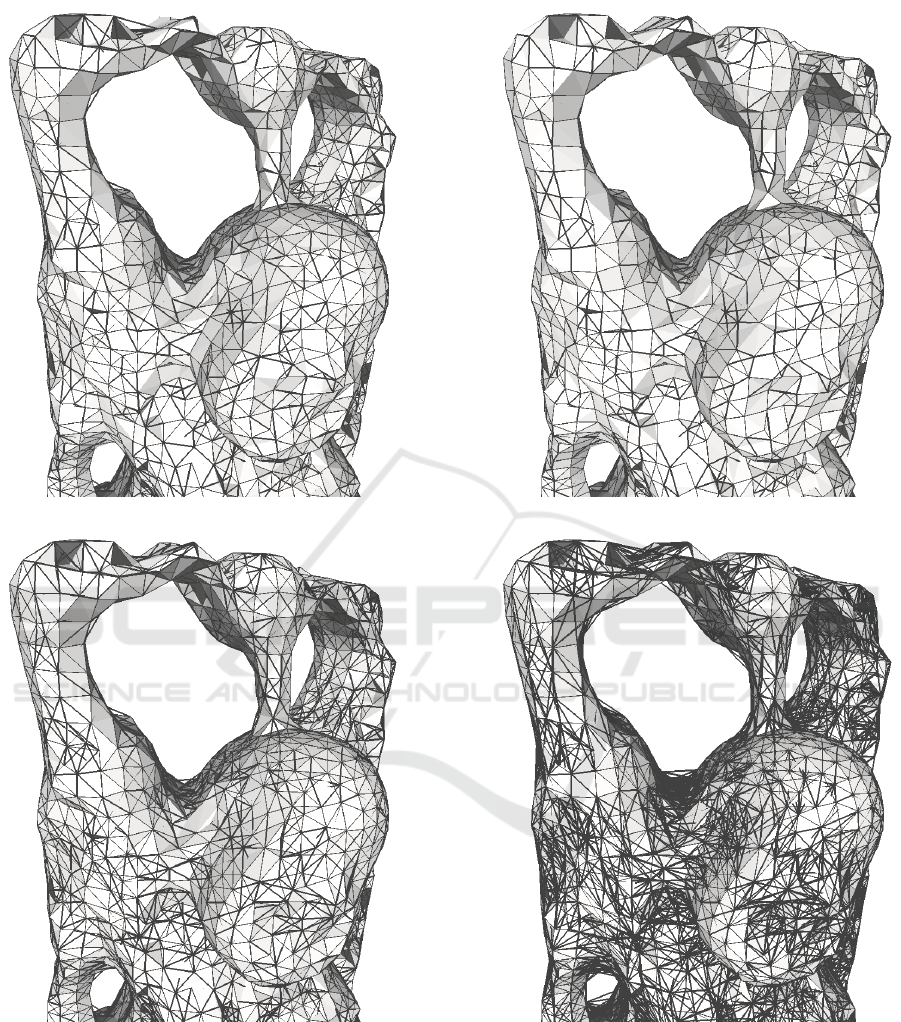
SIG. 6NN.

10NN. 20NN.

Figure 1: Results of our SIG and the kNN graphs for k = {6,10,20} for the connectivity of the Buddha statue from the

Stanford repository. Our graph captures the connectivity well, without many redundant edges, and without the need for a

parameter compared to the kNN graphs. The original surface is shown in light gray, with the various graphs overlaid in black.

Parameter-Free Connectivity for Point Clouds

2 RELATED WORK

Connectivity. Determining the neighborhood of

unstructured points in 3D requires a local descrip-

tion of the points’ relations depending on their dis-

tance. A k-neighbourhood is strongly inﬂuenced by

the choice of the parameter k, which could result in

over-smoothing if the covered area is too large, or

sensitivity to noise for small areas. Hence, picking

a value depends heavily on the particular type of data

and how it is sampled. Being able to choose k usu-

ally requires more time to ﬁnd a suitable value, but it

allows the freedom of dealing with varied data types.

Various subsets of the Delaunay triangulation can

be used as connectivity graphs, such as the rel-

ative neighborhood graph, the Gabriel Graph, the

α-complex (Edelsbrunner et al., 1983), and the β-

skeleton (Kirkpatrick and Radke, 1985). For an edge

pq to exist in the relative neighborhood graph, there

cannot exist another point r that is closer to p or q

than they are to each other. In the Gabriel graph, two

points - p,q, are connected if the closed disc with di-

ameter pq, passing through p and q, contains no other

samples. The α-complex contains all simplices of the

Delaunay triangulation that can be enclosed with a

circle of radius 1/α, empty of other samples. The

β-skeleton has been introduced as a scale-invariant

version of α-shapes, where the edge pq is part of

the graph if angles prq are bound by a threshold - β.

However, we do not include these graphs in our eval-

uation, since, as subsets of the Delaunay triangula-

tion (Jaromczyk and Toussaint, 1992b), they are com-

puted by pruning the triangulation, which is slower

than both kNN and SIG computations. Furthermore,

since the triangulation computation is a prerequisite

for these methods, one could directly reconstruct the

surface, bypassing the need for a proximity graph.

Normal Estimation. An important application of

connectivity retrieval is represented by normal esti-

mation. Normal estimation for point clouds has been

a heavily researched area of computer graphics, as

it usually represents a ﬁrst step or requirement in

surface reconstruction, e.g., for Poisson reconstruc-

tion (Kazhdan et al., 2006) or data-driven approaches

such as Point2Surf (Erler et al., 2020). One of the ba-

sic methods for computing normals for unstructured

point clouds is using Principal Component Analysis

(PCA). This method considers a local patch of ver-

tices and ﬁnds the axis of variance with the least

amount of variance since the points should vary the

least in the normal direction. The relation between

neighborhood choice and normal estimation has been

extensively studied (Mitra and Nguyen, 2003). Other

methods improve on the tangent plane estimation by

using a weighted approach when considering the local

neighborhood (Pauly et al., 2003) or by ﬁtting alge-

braic spheres (Guennebaud and Gross, 2007). How-

ever, these methods all require a good parameter for

choosing an appropriate neighborhood size, which we

do not need with our simple parameter-free method.

Another avenue for estimating normals for point

clouds has been developed with the concept of

poles (Amenta and Bern, 1999). This method is based

on computing the Voronoi diagram on the input points

and extracting the normals as the line connecting each

sample point and the farthest Voronoi vertex to their

Voronoi cell (the pole). This method is sensitive to

noise, but it has been improved to handle noisy sam-

ples (Dey and Goswami, 2006) where it requires ad-

ditional parameters.

Data-Driven Approaches. Recently, multiple data-

driven approaches have been developed, which usu-

ally take advantage of large data repositories to learn

the geometric relations between the point clouds’

structure and their expected normals. Here (Boulch

and Marlet, 2016), they are using a Hough transform

to estimate normals. PCPNet (Guerrero et al., 2018)

builds on the PointNet architecture (Charles et al.,

2017) and uses local patches to estimate the properties

of point clouds with various noise levels and sampling

densities. However, these types of methods require a

long processing time and possible re-training depend-

ing on the type of data.

An alternative to dealing with noise in the ex-

isting point clouds is to ﬁrst denoise them and then

use a connectivity/normal computation approach that

works well on clean data. In this direction, data-

driven approaches have been dealing with noise in

(Rakotosaona et al., 2020), where they build on PCP-

Net to classify outliers and then reproject noisy sam-

ples on the original surface. (Luo and Hu, 2021) use

a noisy point distribution model to estimate scores

and the direction of the surface. Classical, analytical

approaches for denoising include ﬁltering in various

forms, such as the bilateral ﬁlter that takes normals

into account (Digne and de Franchis, 2017) or voting

schemes for feature detection that later help in normal

repositioning (Liu et al., 2020). This kind of prepro-

cessing could enable our method to also connect noisy

point clouds since it is designed as an interpolating

method to recover the connectivity.

Moreover, connectivity retrieval has applications

in other data-driven approaches. Methods that use

graph convolutional neural networks on point clouds

for various purposes, such as reconstruction or seg-

mentation, create a graph on the input points (and

GRAPP 2024 - 19th International Conference on Computer Graphics Theory and Applications

sometimes on the deeper layers of the network as

well) and use it to learn about the data and infer the

surface or various labels on the input points (Shi and

Rajkumar, 2020; Wang et al., 2019). Usually, they use

kNN or a ﬁxed radius neighbor search as their con-

nectivity encoding, which could be replaced by our

method to improve results.

Spheres-of-Inﬂuence. The spheres-of-inﬂuence

graph (SIG) has been introduced as a clustering

method (Toussaint, 1988). Two vertices are con-

nected in the SIG if their distance is less or equal to

the sum of the distances to their respective nearest

neighbors. This graph was previously used for

estimating local densities for surface reconstruc-

tion (Klein and Zachmann, 2004), but our method

aims to recover connectivity, not a surface. Moreover,

the rarely used SIG has recently gotten attention

in reconstruction methods (Marin et al., 2022; de

Figueiredo and Paiva, 2022) where combined with

the Delaunay graph it showed promising results for

curve and region reconstruction.

3 METHOD

We deﬁne a mesh as a collection of ver-

tices - V = {p ∈ R

} and triangulated faces -

T = {(a,b, c)|a,b, c ∈ V,a ̸= b ̸= c ̸= a}. Using

only the set of unstructured points V = {p ∈ R

we aim to recover a set of edges that connect the

given samples as similar as possible to the original

connectivity of the mesh which is encoded in T . We

deﬁne similarity here as edge connectivity, instead

of the exact triangulation of the original mesh. Our

method uses the spheres-of-inﬂuence graph, and we

provide an improved algorithm to efﬁciently compute

this proximity graph. We are using the vertices of

triangulated meshes as our input in order to have

access to a ground truth connectivity to which we can

compare our results.

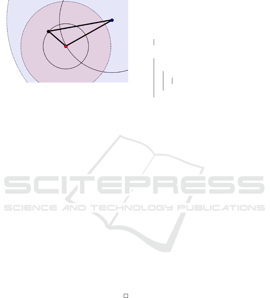
Spheres-of-Inﬂuence Graph. The SIG contains all

the edges (v

) such that for their respective end-

points, v

and v

, the following holds:

∥v

∥ ≤ nn(v

) + nn(v

), (1)

where ∥a,b∥ represents the Euclidean distance be-

tween points a and b, and nn(a) represents the dis-

tance between a and its nearest neighbor. This con-

dition can be interpreted visually as centering a ball

at each vertex, with radius equal to the distance to

the nearest neighbor of that vertex, and connecting

all points whose balls intersect, as it can be seen in

Figure 2. This graph encodes the spatial proximity of

vertices well, without the need for a parameter. It con-

tains the Nearest Neighbor graph (Toussaint, 1988),

as the edge between points and their respective near-

est neighbor will always satisfy the condition.

Figure 2: Visual representation of the SIG connectivity - the

intersections of circles generate the set of SIG edges.

Various properties of the sphere-of-inﬂuence

graph have been investigated, such as the bound on

the size of the graph (Dwyer, 1995) or its behav-

ior under different metric spaces (Michael and Quint,

1999). However, even if the number of edges has been

proven to be linear, algorithms to efﬁciently compute

the graph have not yet been researched, especially

considering that SIG is not included in the Delaunay

triangulation and hence, the latter cannot be used as a

starting point for pruning (Jaromczyk and Toussaint,

1992a). We show that the neighbors of each vertex in

SIG are bounded inside a ﬁxed radius - Figure 3, and

we use this spatial constraint to improve the speed of

the computation.

Theorem 1. For all vertices a ∈ V , all SIG edges

(a,b),b ∈ V,a ̸= b, are contained in a radius of at

most 2nn(a) from a or in a radius of at most 2nn(b)

from b, where nn(v) is the distance between v and its

nearest neighbor, for v ∈ V .

Proof. We will prove the statement by contradiction.

Let us compute the distance to the nearest neighbor

for each vertex and store the result as nn(v) for all

vertices v ∈ V . For each vertex v, retrieve all the ver-

tices within 2nn(v) distance of v and only store the

edges that satisfy the SIG criterion. Let us call the

obtained graph FastSIG (FSIG).

Since we are trying to prove Theorem 1 by con-

tradiction, we assume that there exists at least an edge

that is outside the range boundaries we have deﬁned

(within 2nn(a) for each vertex). This means that there

has to exist an edge (a, b) which is in SIG but not in

Parameter-Free Connectivity for Point Clouds

Figure 3: We illustrate the spheres of inﬂuence of vertices

a and b in 2D as outlined circles, with a radius equal to the

distance to their respective nearest neighbor. The bound-

ing radius of the incident SIG edges are colored disks with

dashed borders of radius equal to twice the SIG radius. We

can observe that even if b is not in the incidence radius of

a, a is contained in b’s radius, showing that SIG edges are

contained in at least one of the endpoints’ incidence radii.

FSIG. Hence,

∥a,b∥ ≤ nn(a) + nn(b), (2)

since (a,b) ∈ SIG and

∥a,b∥ > 2nn(a), (3)

from (a,b) ̸∈ FSIG, while checking a’s neighbours

which do not include b and

∥b,a∥ > 2nn(b), (4)

from (a,b) ̸∈ FSIG, while checking b’s neighbours

which do not include a. Summing the last two equa-

tions, we get:

2∥a,b∥ > 2nn(a) + 2nn(b), (5)

since ∥a,b∥ = ∥b, a∥. Dividing by 2, we get:

∥a,b∥ > nn(a) + nn(b), (6)

which contradicts our assumption of (a, b) ∈ SIG.

Since we have arrived at a contradiction, we have

proved that all SIG edges are in FSIG as well.

Having proved that SIG edges live in a ﬁxed

boundary from every node, we use this information

to retrieve all the neighboring nodes within the given

radius using a kdtree, as presented in Algorithm 1.

4 RESULTS

We are aiming to provide an alternative for kNN that

is parameter-free, fast to compute, efﬁcient to store,

Data: V = {v ∈ R

}

Result: SIG={(a,b) : a, b ∈ V,a ̸= b,||a,b|| ≤

nn(a) + nn(b)}

SIG={};

create kd-tree KT of V ;

for v ∈ V do

ﬁnd nn(v) using KT ;

end

for v ∈ V do

N = KT .ﬁndNbrInRange(2nn(v));

for u ∈ N do

if ||u,v|| ≤ nn(u) + nn(v) then

SIG += (u,v);

end

Algorithm 1: Fast SIG computation.

and achieves better or similar surface properties to

kNN for a wide variety of data. In this section, we will

show how SIG satisﬁes all these requirements, repre-

senting a good, parameter-free alternative to kNN for

estimating unstructured point clouds’ connectivity.

We have tested our method on a varied dataset

of points clouds exhibiting various features, such as

various types of non-uniform sampling and sharp

edges. We compared our results to the kNN neigh-

borhood for connectivity recovery, for usual values

of k = {6,10, 20}. We did not use k-values lower

than 6 since this is the average degree of vertices in

triangulated meshes, as can be shown using Euler’s

formula. As an application, we have also computed

normals using PCA from our graph and from the

kNN graphs and compared these with the face-based

normals of the original meshes.

Dataset. We have used a subset of the

Thingy10K (Zhou and Jacobson, 2016) dataset

of meshes that are manifold and have less than 1k

vertices for our quantitative results, consisting of

around 3k different models. Most of these meshes

exhibit CAD-like features in the form of having

samples mainly along edges, with thin and long

faces. This type of sparse sampling affects the

results of our connectivity measures, as, on average,

none of the investigated connectivity graphs can

perfectly capture the original connectivity, but we

have chosen to include this type of data as well to test

the resilience of our method in the presence of sparse

sampling. For qualitative results, we have included

some of the meshes from the Stanford repository

(https://graphics.stanford.edu/data/3Dscanrep/) -

the resulting graphs using the Stanford bunny are

presented in Figure 4.

GRAPP 2024 - 19th International Conference on Computer Graphics Theory and Applications

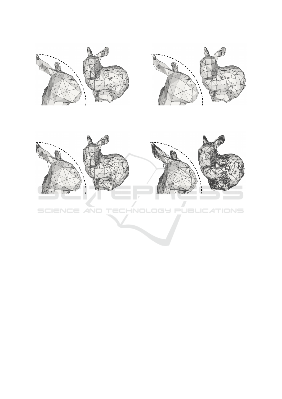
(a) SIG edges computed for the Stanford bunny. The

edges mostly follow the original triangulation, with ad-

ditional diagonals, but without any edges that incorrectly

connect the input samples.

(b) 6NN graph of the Standford bunny. The close-up

shows that not all edges of the face are captured, but ad-

ditional edges appear close to the ears.

are visible around the ears.

(d) 20NN graph of the input points. Many redundant

edges are visible on the ears and the body.

Figure 4: Results of our graph and kNN for k = {6, 10, 20} on the Stanford bunny, where the original surface is presented in

gray, with various connectivity graph edges overlaid in black.

Connectivity. The connectivity of the ground truth

is what our graph aims to reconstruct. However, the

original edge set is not a unique representation of the

intrinsic connectivity of points, as it is highly depen-

dent on the chosen triangulation, e.g., edges may ﬂip,

as can be visible in Figure 5. Hence, we do not aim to

reproduce the exact edges of the ground truth meshes

(i.e., comparing the 1-ring of each vertex), but to cre-

ate a good approximation of the connectivity of the

entire surface.

In order to quantify how close our graph is to

the original connectivity, we used the DeltaCon met-

ric (Koutra et al., 2016), where a value of 0 means

the graphs are completely different and a score of 1

implies identical graphs. DeltaCon computes a ma-

trix of node-to-node inﬂuence for each graph and the

ﬁnal score is a difference between these two n

matri-

ces. This is equivalent to using m-ring neighborhoods

(m ∈ [1,n]) for each vertex with decreasing weights

as we move farther from the current node. Moreover,

this metric beneﬁts from edge awareness - discon-

necting changes are penalized more than removing an

edge from a complete graph, and this is a property that

highly inﬂuences the type of connectivity we want to

measure for our method. For a detailed deﬁnition of

the metric and its implementation, we direct to the

original works (Koutra et al., 2016).

We have computed DeltaCon for the initial 3431

meshes from Thingy10K, with various numbers of

vertices and different sampling densities. The results

are presented in Figure 6, where SIG consistently ob-

tains higher scores than the kNN graphs. The re-

sults are clustered in equally sized buckets depend-

ing on the number of vertices. For each bucket, we

present the averaged DeltaCon measurement over all

inputs with the total number of vertices in the spec-

iﬁed range. Even if the metric does not achieve 1,

as the graphs are not identical (as we do not aim for

this), our graph manages to encode the original con-

nectivity better than the kNN graphs. The maximum

DeltaCon value achieved by all methods is also lower

than 1 due to the sparse sampling of the dataset, as

mentioned previously.

Parameter-Free Connectivity for Point Clouds

Figure 5: Local changes in the triangulation choice - such as edge ﬂips, do not affect the overall connectivity of the mesh.

The four highlighted vertices create the same connected surface in both ﬁgures.

Figure 6: DeltaCon graph similarity metric - a higher value

corresponds to a closer similarity to the original graph.

Storage. Low storage represents another requirement

for our method, since we try to use the minimum

amount of edges that preserve the connectivity by

making use of the spatial proximity properties of SIG.

The total number of edges for each graph can be seen

in Figure 7, where the results are presented with re-

spect to the number of vertices. Our method achieves

the lowest number of edges and hence, has the lowest

storage requirement. Our number of edges is lower

than the ground truth since the ground truth number

of edges is extracted from triangulated meshes, which

contain some redundant edges with respect to connec-

tivity.

Surface Approximation: Geodesic. We are also

comparing the distance between pairs of nodes in our

graph to the geodesic distance over the ground truth

surface, computed using the Heat Method (Crane

et al., 2017). This way, we measure how close the

graph edges follow the surface. For all pairs of nodes

in the original mesh, we compute the ratio between

the geodesic distance over the original mesh and the

shortest distance between the same nodes in SIG and

between the same nodes in the kNN graphs. The re-

Figure 7: Number of edges in graphs plotted against the

number of vertices. We consistently obtain the smallest

number of edges by a large margin, while still correctly pre-

serving the original connectivity.

sults are shown in Figure 8, where we present the ratio

of distances in relation to the number of vertices in the

input. The differences between buckets are due to the

varying number of input datasets in each bucket, as

well as the type of meshes - a single mesh with close

sheets and sparse sampling, such as the one presented

in Figure 9 highly increases the error for the connec-

tivity graphs. We aim to obtain a resulting ratio of

1, as values lower than 1 indicate longer paths in the

proximity graphs, while values higher than 1 would

imply the existence of shortcuts (too many edges) in

the connectivity graphs. Our method is consistently

close to the desired ratio of 1 across the tested meshes,

without the need to tune any parameters. Even if

for some of the tested input ranges some of the kNN

graphs have better results, these are not universal and

the user would need to adjust k depending on the us-

age, which is an issue solved by our method.

Application: Normal Estimation. We propose SIG

as a connectivity graph that encodes surface proper-

ties well, and can act as an alternative for the com-

monly used kNN graphs. One usual application is

GRAPP 2024 - 19th International Conference on Computer Graphics Theory and Applications

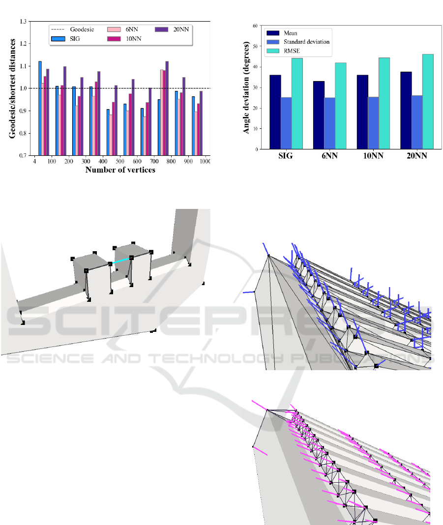
Figure 8: Ratio of the geodesic distance traced on the sur-

face to the shortest path in the computed graph, ideally 1.

Figure 9: Sparse sampling of close sheets (the parallel

tower-like structures in the center) generates edges across

the surface. These skew our measurement of the geodesic

ratio to the shortest distance, as the surface originally fol-

lows the U-structure, while our graph shortcuts it through

the edge connecting the two towers, highlighted in blue.

However, similar behavior is exhibited by the kNN graphs,

since all of them are distance-based.

normal computation for unstructured point clouds us-

ing PCA. Even though more advanced normal com-

putation methods have been developed, constructing

them using PCA on a connectivity graph still repre-

sents a widely used method and good results in this

direction indicate an overall good representation of

the underlying surface. Moreover, we are not aiming

to improve the normal computation in general, but to

show that our graph can be used in similar applica-

tions as kNN.

For each vertex, we computed the covariance

matrix using its neighbors and extracted the normal

as the normalized eigenvector corresponding to the

smallest eigenvalue. We do not consistently orient

the normals, as this can be done in a post-processing

step and we are only interested in the angle difference

Figure 10: Angle variation between normals computed us-

ing PCA over connectivity graphs and original, face-based

normals. We compute the mean and the standard deviation

of the angle difference, and the root mean square error. All

of the methods achieve similar deviations. The overall error

is high due to the sharp angles in the input dataset.

(a) Ground-truth normals computed using the incident

faces of each vertex.

(b) Normals computed with PCA using the SIG con-

nectivity. The sparse sampling creates parallel lay-

ers and normals are oriented accordingly since the top

vertices do not get connected across layers. However,

this is an issue encountered by distance-based meth-

ods in general.

Figure 11: Example of how CAD-like models with sparse

sampling affect the computed connectivity, and hence, the

normal computation.

Parameter-Free Connectivity for Point Clouds

(a) Ground-truth normals computed using the incident

faces of each vertex.

(b) PCA normals computed using SIG are very close

to the ground truth. Normals are computed for every

vertex, but since we do not orient them consistently,

some of them are facing the other way and are not

visible. Note that for our evaluation, orientation does

not matter, and consistency is usually achieved with a

post-processing step.

Figure 12: Improved normal computation of our method for

more uniformly sampled meshes.

when compared to the ground truth, which can

be computed without the consistent orientation.

For the original meshes, we used the triangulated

faces to compute the normals. We do not use the

ground truth edge graph since that would bias the

normal computation in the direction of a speciﬁc

triangulation. Instead, face-based normal computa-

tion takes into account more information about the

surface, and not only a speciﬁc 1-ring. Then, we

computed the average angle deviation for SIG and

the kNN graphs when compared to the ground truth

normals. Results are presented in Figure 10, where

the difference among the various tested graphs is less

than 1 degree for all the metrics. Since the chosen

dataset contains surfaces that are sparsely sampled,

the normal computation achieved high errors for

all graphs. Thus, for this metric, we resampled the

chosen dataset (adding new vertices along edges

longer than a speciﬁed threshold and retriangulating),

obtaining models with up to 7k vertices. An example

of how sparse sampling, which is also an issue in

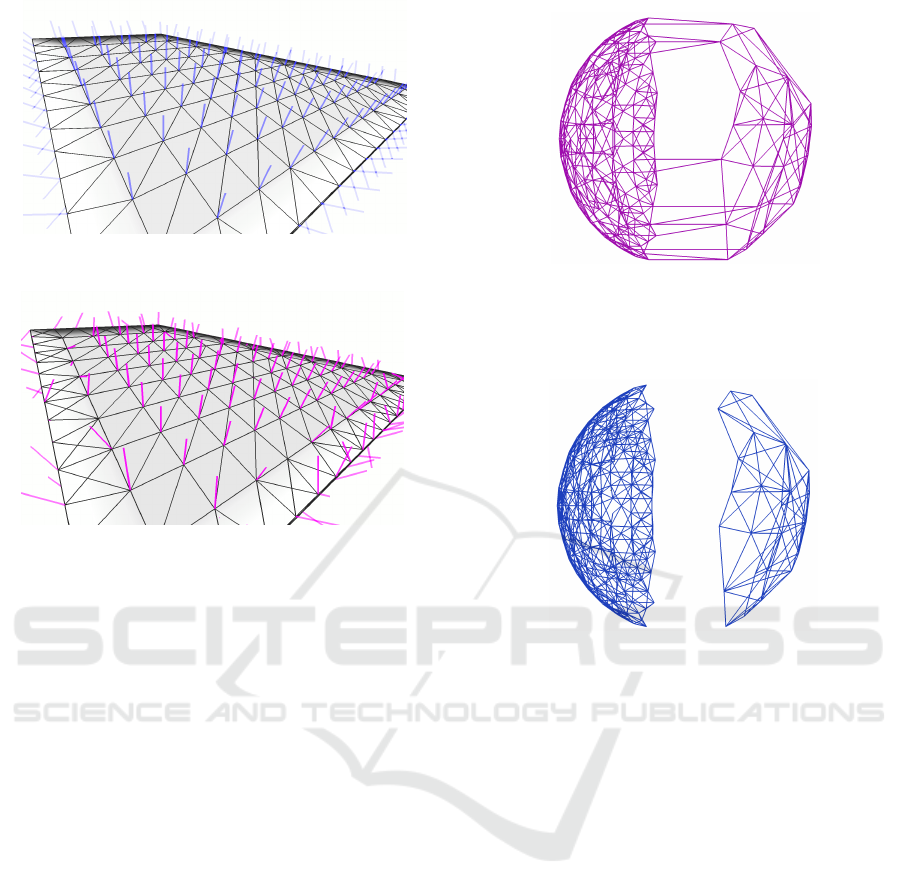
LIDAR scans, can cause problems, is presented in

(a) 6NN creates bridges between the two hemi-

spheres, since the graph does not consider local densi-

ties. Increasing the k value only aggravates the issue,

as more bridge edges will be constructed.

(b) SIG only creates edges on each hemisphere, with-

out crossing the gap between the two surface sheets.

Figure 13: Different sampling densities on two surface

sheets that are close together - the two hemispheres are not

connected as ground truth.

Figure 11, where there is not enough information

for the vertices placed on edges to have their normal

computed correctly. However, for well-sampled

models, the normals are close to the ground truth -

Figure 12. The overall angle deviation is still high

for all methods, since some of the meshes exhibit

sharp angles, for which the normal computation is

also erroneous for all graphs.

Timings. Due to the proved bounded radius in which

SIG neighbors are found, our method’s timings are

comparable to kNN, as can be observed in Figure 14.

We observe a linear increase in the computational

time with the number of vertices, which is expected

due to the linear nature of our algorithm. Our method

is only slightly slower than 6NN, but achieves better

results overall and manages to do so with many fewer

edges.

All experiments have been performed using

an AMD Ryzen 7 5800 processor. Both kNN

and SIG graphs have been implemented using the

GRAPP 2024 - 19th International Conference on Computer Graphics Theory and Applications

100

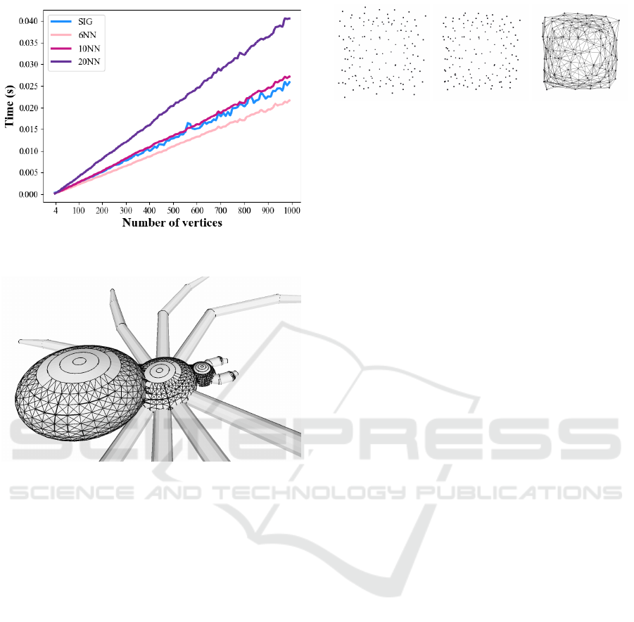
Figure 14: Timings of our method compared to kNN graphs

for inputs with various numbers of vertices.

Figure 15: Parallel layers of sampling result in disconnected

ring-like structures as can be observed on the spider’s body

and legs. However, kNN graphs exhibit similar issues if the

sampling is too sparse and nodes are clustered in layers.

scipy.spatial.KDTree in python.

Limitations. Since our method depends on distances,

non-uniform sampling may negatively affect the re-

sult, as is commonly the case with connectivity re-

construction. An example can be seen in Figure 15,

where the spider’s legs and top of the body are uni-

formly sampled along parallel layers. For real-world

point clouds, LIDAR scans can produce such arti-

facts. These conﬁgurations are difﬁcult to handle for

all methods, as they may fail to connect subsets of

the point cloud. Such issues could be mitigated by

employing an incremental SIG - using the next near-

est neighbors until a speciﬁc vertex degree or average

neighbor angle has been reached for the current graph.

However, in the case of different sampling densi-

ties on distinct parts of the same object, our method

has an advantage over kNN. Our method is less likely

to create edges between surface sheets that are geo-

metrically close, but geodesically distant (Figure 13).

(a) Noisy. (b) Denoised. (c) SIG.

Figure 16: Denoising pipeline that would allow our method

to give good results on noisy point clouds. The noisy point

cloud of a cube is denoised in 16b using the Bilateral Fil-

ter (Digne and de Franchis, 2017), and then used as input

for our SIG computation, resulting in a graph that closely

approximates the original cube.

Our method is not robust to noise by design, as

it computes a distance-based neighborhood, exhibit-

ing similar drawbacks as kNN graphs. Noisy point

clouds could still be used with our method, provided

they have been cleaned in a pre-processing step us-

ing, for example, PointCleanNet (Rakotosaona et al.,

2020), the Bilateral Filter (Digne and de Franchis,

2017) or Score-Based Denoising (Luo and Hu, 2021),

as demonstrated in Figure 16.

5 CONCLUSIONS

We present an alternative to the commonly used

kNN graphs for establishing the connectivity of point

clouds: the SIG, a parameter-free proximity graph. In

our work, we introduce novel spatial constraints for

the extent of SIG edges, leveraging this new property

to enhance its computational efﬁciency. We demon-

strate the SIG’s improved connectivity representation

that is parameter-free. Moreover, as a sparse graph,

it has a lower edge count, thus minimizing storage

requirements. Consequently, it offers three key

advantages over kNN: no need for parameter tuning,

sparsity, and improved connectivity encoding. As an

incidental application, we have shown that computed

normals are of competitive quality to kNN.

Future Work. We aim to utilize the advantage of

parameter-free improved connectivity for surface re-

construction. Moreover, we are planning to use the

SIG neighborhood (with possible extensions to n

nearest neighbor) in graph-convolutional networks for

learning from 3D point cloud data. We also plan to in-

vestigate how our method can create an advantage in

other ﬁelds, such as motion planning and simulations.

Parameter-Free Connectivity for Point Clouds

101

ACKNOWLEDGMENTS

This work has been partially funded by the Austrian

Science Fund (FWF) project no. P32418-N31 and

by the Wiener Wissenschafts-, Forschungs- und Tech-

nologiefonds (WWTF) project ICT19-009.

REFERENCES

Amenta, N. and Bern, M. (1999). Surface reconstruction by

voronoi ﬁltering. Discr. & Comp. Geom., 22:481–504.

Boulch, A. and Marlet, R. (2016). Deep learning for ro-

bust normal estimation in unstructured point clouds.

Computer Graphics Forum, 35(5):281–290.

Charles, R. Q., Su, H., Kaichun, M., and Guibas, L. J.

(2017). Pointnet: Deep learning on point sets for 3d

classiﬁcation and segmentation. In 2017 IEEE CVPR,

pages 77–85.

Crane, K., Weischedel, C., and Wardetzky, M. (2017).

The heat method for distance computation. Commun.

ACM, 60(11):90–99.

de Figueiredo, L. H. and Paiva, A. (2022). Region recon-

struction with the sphere-of-inﬂuence diagram. Com-

puters & Graphics, 107:252–263.

Dey, T. K. and Goswami, S. (2006). Provable surface recon-

struction from noisy samples. Computational Geom-

etry, 35(1):124–141. Special Issue on the 20th ACM

Symposium on Computational Geometry.

Digne, J. and de Franchis, C. (2017). The bilateral ﬁlter for

point clouds. Image Processing On Line, 7:278–287.

Dwyer, R. A. (1995). The expected size of the sphere-of-

inﬂuence graph. Comp. Geometry, 5(3):155–164.

Edelsbrunner, H., Kirkpatrick, D., and Seidel, R. (1983).

On the shape of a set of points in the plane. IEEE

Transactions on Information Theory, 29(4):551–559.

Erler, P., Guerrero, P., Ohrhallinger, S., Mitra, N. J., and

Wimmer, M. (2020). Points2surf learning implicit sur-

faces from point clouds. In Computer Vision–ECCV

2020, Proceedings, Part V, pages 108–124. Springer.

Guennebaud, G. and Gross, M. (2007). Algebraic point set

surfaces. ACM Trans. Graph., 26(3):23–es.

Guerrero, P., Kleiman, Y., Ovsjanikov, M., and Mitra,

N. J. (2018). Pcpnet learning local shape properties

from raw point clouds. Computer Graphics Forum,

37(2):75–85.

Jaromczyk, J. and Toussaint, G. (1992a). Relative neigh-

borhood graphs and their relatives. Proceedings of the

IEEE, 80(9):1502–1517.

Jaromczyk, J. W. and Toussaint, G. T. (1992b). Relative

neighborhood graphs and their relatives. Proc. IEEE,

80:1502–1517.

Kazhdan, M., Bolitho, M., and Hoppe, H. (2006). Poisson

Surface Reconstruction. In Symposium on Geometry

Processing. The Eurographics Association.

Kirkpatrick, D. G. and Radke, J. D. (1985). A framework

for computational morphology. Machine Intelligence

and Pattern Recognition, 2:217–248.

Klein, J. and Zachmann, G. (2004). Point cloud surfaces us-

ing geometric proximity graphs. Computers & Graph-

ics, 28(6):839–850.

Koutra, D., Shah, N., Vogelstein, J. T., Gallagher, B., and

Faloutsos, C. (2016). Deltacon: Principled massive-

graph similarity function with attribution. ACM Trans.

Knowl. Discov. Data, 10(3).

Liu, Z., Xiao, X., Zhong, S., Wang, W., Li, Y., Zhang, L.,

and Xie, Z. (2020). A feature-preserving framework

for point cloud denoising. Computer-Aided Design,

127:102857.

Luo, S. and Hu, W. (2021). Score-based point cloud denois-

ing. In 2021 ICCV, pages 4563–4572.

Marin, D., Ohrhallinger, S., and Wimmer, M. (2022). Sigdt:

2d curve reconstruction. CGF, 41(7):25–36.

Michael, T. and Quint, T. (1999). Sphere of inﬂuence graphs

in general metric spaces. Mathematical and Computer

Modelling, 29(7):45–53.

Mitra, N. J. and Nguyen, A. (2003). Estimating surface

normals in noisy point cloud data. In Proceedings of

the Nineteenth Annual Symposium on Computational

Geometry, SCG ’03, page 322–328, New York, NY,

USA. Association for Computing Machinery.

Pauly, M., Keiser, R., Kobbelt, L., and Gross, M. (2003).

Shape modeling with point-sampled geometry. ACM

SIGGRAPH 2003 Papers, SIGGRAPH ’03.

Rakotosaona, M.-J., La Barbera, V., Guerrero, P., Mitra,

N. J., and Ovsjanikov, M. (2020). Pointcleannet:

Learning to denoise and remove outliers from dense

point clouds. Comp. Graph. Forum, 39(1):185–203.

Shi, W. and Rajkumar, R. (2020). Point-gnn: Graph neural

network for 3d object detection in a point cloud. In

Proc. of the IEEE/CVF conference on computer vision

and pattern recognition, pages 1711–1719.

Toussaint, G. T. (1988). A graph-theoretical primal sketch.

In Machine Intelligence and Pattern Recognition, vol-

ume 6, pages 229–260. Elsevier.

Wang, L., Huang, Y., Hou, Y., Zhang, S., and Shan, J.

(2019). Graph attention convolution for point cloud

semantic segmentation. In 2019 CVPR, pages 10288–

10297.

Zhou, Q. and Jacobson, A. (2016). Thingi10k: A dataset of

10,000 3d-printing models. arXiv:1605.04797.

GRAPP 2024 - 19th International Conference on Computer Graphics Theory and Applications

102