Efﬁcient Solver Scheduling and Selection for Satisﬁability Modulo

Theories (SMT) Problems

David Moj

sek

and Jan H

ula

University of Ostrava, 30. dubna 22, 702 00 Ostrava, Czech Republic

Keywords:

Satisﬁability Modulo Theories (SMT), Solver Scheduling, Algorithm Selection, Dynamic Scheduling.

Abstract:

This paper introduces innovative concepts for improving the process of selecting solvers from a portfolio to

tackle Satisﬁability Modulo Theories (SMT) problems. We propose a novel solver scheduling approach that

signiﬁcantly enhances solving performance, measured by the PAR-2 metric, on selected benchmarks. Our

investigation reveals that, in certain cases, scheduling based on a crude statistical analysis of training data

can perform just as well, if not better, than a machine learning predictor. Additionally, we present a dynamic

scheduling approach that adapts in real-time, taking into account the changing likelihood of solver success.

These ﬁndings shed light on the nuanced nature of solver selection and scheduling, providing insights into

situations where data-driven methods may not offer clear advantages.

1 INTRODUCTION

We are introducing a series of innovative concepts and

reﬁnements to the process of selecting solvers from a

portfolio to solve problems of Satisﬁability Modulo

Theories (SMT). Our methodology exhibits similari-

ties to MachSMT (Scott et al., 2021), albeit with the

potential for superior performance in various opera-

tional scenarios. Furthermore, we show that in many

cases trained Machine Learning (ML) model can be

omitted and one can even ignore features of problem

at hand and simply run the same schedule, designed

on training set, for all testing examples. As an illus-

trative case, we have chosen the scheduling of SMT

solvers, but it is essential to underscore that our pro-

posed techniques are universally applicable to situa-

tions where algorithm selection from a diverse port-

folio is a requisite.

The central emphasis of our approach revolves

around comparing the trained machine learning algo-

rithm and the scheduling approach without any train-

ing. Importantly, the role of this algorithm is not

merely to identify a single best solver for a given

problem but rather to construct an efﬁcient sched-

ule similar to (Pimpalkhare, 2020). When creating

this schedule, we consider the interaction between the

solving capabilities of different algorithms.

https://orcid.org/0000-0002-3867-644X

https://orcid.org/0000-0001-7639-864X

This consideration is crucial, as it helps us steer

clear of scenarios where two algorithms, capable of

solving the same class of problems, also share a

propensity for failure on similar examples, when run

consecutively.

Our contribution comprises two key parts. First,

we propose a novel solver scheduling approach that

signiﬁcantly improves the PAR-2 metric in selected

benchmarks. Second, we explore the necessity of

employing a ML predictor. Our investigation reveals

that, in certain cases, scheduling based on crude sta-

tistical analysis of training data performs just as well,

if not better, than an ML predictor. The superiority

of this scheduling is clearly visible especially in case

when it competes against a single selected solving al-

gorithm. These ﬁndings highlight the nuanced nature

of solver selection and scheduling, shedding light on

instances where machine learning methods do not of-

fer clear advantages.

2 PRELIMINARIES

2.1 Domain Description - Satisﬁability

Modulo Theories

The SMT-LIB standard (Barrett et al., 2010) deﬁnes

the language and standardized theories. A reposi-

tory of benchmark problems is maintained within the

360

Mojžíšek, D. and H ˚ula, J.

Efﬁcient Solver Scheduling and Selection for Satisﬁability Modulo Theories (SMT) Problems.

DOI: 10.5220/0012393600003654

Paper published under CC license (CC BY-NC-ND 4.0)

In Proceedings of the 13th International Conference on Pattern Recognition Applications and Methods (ICPRAM 2024), pages 360-369

ISBN: 978-989-758-684-2; ISSN: 2184-4313

( set−log ic UFNIA )

( declare−fun f ( I n t ) I n t )

( declare−const c I n t )

( assert (= ( f c ) 0 ) )

( assert

( f o r a l l ( ( x I n t ) ) (>= ( f x ) (

c ( f x ) ) ) ) )

( check−sat )

Figure 1: Example SMT input using the UFNIA logic.

SMT-LIB framework (Barrett et al., 2016). In this

context, a combination of theories is referred to as a

”logic.” For example, logic UFNIA encompasses un-

interpreted functions (theory UF) and non-linear in-

teger arithmetic (theory NIA). Hence, it is mandatory

for each problem ﬁle to specify the intended logic in

the header.

The SMT input format employs a notation similar

to that of LISP. An illustrative example is provided in

Figure 1, featuring an uninterpreted (unknown) func-

tion, denoted as f , mapping integers to integers, and

an uninterpreted integer constant, c. The formula

comprises two ”assertions” which are essentially sub-

formulas that must hold. The initial assertion stip-

ulates that f must yield a result of 0 when applied

to c, while the second assertion demands that f (x)

must be greater than or equal to c f (x) for any integer

x. This example problem is categorized as non-linear

due to the presence of a multiplication operation be-

tween two unknowns.

The command check-sat instructs the solver to as-

sess the satisﬁability of the previously stated asser-

tions. In the case of this example problem, it can be

trivially satisﬁed, for instance, by keeping f constant

and equal to 0. It is important to note that problems

can contain multiple check-sat statements, but this ar-

ticle’s focus is exclusively on single-query problems.

2.2 SMT Solvers

Satisﬁability Modulo Theories (SMT) solvers are in-

dispensable tools in formal methods, effectively au-

tomating logical reasoning across a multitude of the-

ories and their combinations. They ﬁnd applications

in critical domains, including software and hardware

veriﬁcation, symbolic execution, and constraint solv-

ing (de Moura and Bjørner, 2012), (Godefroid et al.,

2012), (Bjørner and de Moura, 2014). It is worth not-

ing that the performance of different SMT solvers can

vary signiﬁcantly when applied to the same problem

instance. One solver may outperform others in a spe-

ciﬁc instance, while the situation might reverse when

faced with a different problem. This variability is of-

ten linked to the unique features and characteristics of

each problem instance.

This interplay between problem instances and

solver performance underscores the complexity of se-

lecting the most appropriate solver for the problem

at hand. To tackle this challenge, practitioners of-

ten rely on extensive experimentation, benchmark-

ing, and proﬁling of solvers to gain insight into their

strengths and weaknesses. Such insights enable the

development of strategies for effectively matching

problem instances with the most suitable solvers, con-

tributing to more efﬁcient and reliable automated rea-

soning. Understanding these dynamics between prob-

lem features and solver performance is crucial in har-

nessing the full potential of SMT solvers across vari-

ous application areas.

2.2.1 Notable SMT Solvers

It is not a goal to describe all existing solvers, but

for reference we give a few examples of solvers often

recurring in our predictions and schedules.

• Z3. Developed at Microsoft Research (De Moura

and Bjørner, 2008).

• CVC4. Developed jointly by Stanford University

and the University of Iowa (Barrett et al., 2011).

• MathSAT. A joint project of the Fondazione

Bruno Kessler (FBK-irst) and the University of

Trento (Bruttomesso et al., 2008).

• Yices 2. Developed by the Stanford Research In-

stitute (SRI International) (Dutertre, 2014).

2.3 Problem Description

Let S = {s

, . . . , s

} be a set of l SMT solvers that

we have at our disposal. Our goal is to produce

an effective algorithm which on a per-instance ba-

sis creates a schedule from the set S. This means

that we want to ﬁnd a function f

(parameterized by

θ) that takes a representation of an SMT formula q

and the set S as input and outputs an ordered tuple

(q, S) = ((i

), . . . , (i

)) where i

’s are indices

of selected solvers and t

’s are times assigned to these

solvers

. The sum

∑

≤ t

max

is restricted by t

max

which is the maximum time we are willing to spend

solving the problem.

Given a formula q and its schedule f

(q, S), we

measure how long it takes to solve the formula us-

ing this schedule. We denote this measurement by

M(q, f

(q, S)) and set it to a constant number t

pen

Note that this deﬁiton of problem wraps all cases dis-

cussed in our experiments. The schedule with one solver

can correspond to selecting the single best one, and the

greedy schedule treats the selection of the solver as a con-

stant function with respect to the varying input.

Efﬁcient Solver Scheduling and Selection for Satisﬁability Modulo Theories (SMT) Problems

361

(with t

pen

> t

max

) if the formula was not solved within

the time limit t

max

We assume that the problems/formulas we want

to solve come from an unknown distribution P and

that we have a ﬁnite set of independent and identically

distributed samples Q = {q

, . . . , q

} where q

∼ P.

Because the distribution P is unknown, we can

only try to minimize an approximation to the objec-

tive function samples in Q:

∗

= arg min

∑

∈Q

M(q

, f

, S)).

The parameters of this function cannot be directly

optimized with respect to the objective function by

gradient-based methods because it involves discrete

choices.

3 SCHEDULING OF SMT

SOLVER

In this paper, we compare a machine learning model

that selects the best solver for a given problem in-

stance, a dynamic schedule based on this selection,

and a trivial way to schedule solvers without even

looking at the problem. For that reason, we ﬁrst

need to clarify how solvers are ranked with a machine

learning model.

3.1 Interval Prediction

Our predictor is inspired by the Empirical Hardness

Model (EHM) (Leyton-Brown et al., 2009) used in

MachSMT. For each logic and solver combination,

we train a dedicated model to predict the runtime re-

quired for that solver to solve an SMT problem in-

stance based on its features. The key change here is

that we don’t directly train the EHM. Instead, we di-

vide the runtime into multiple indexed intervals repre-

sented as I = (i

, i

, ..., i

), deﬁned by their endpoint

values t(i

). Our goal is to predict in which of these

intervals the solver will complete the instance. This

transformation turns the regression task into a classi-

ﬁcation problem.

We explored various methods to divide the run-

time into intervals. It is crucial to consider that most

instances are either solved very quickly or remain un-

solved. A uniform split would result in unbalanced

classes. We found that using a power or exponential

function for splitting worked better, but also left us

with empty classes. Ultimately, we opt for creating

perfectly balanced classes by using quantiles derived

from the solving times of the speciﬁc solver on in-

stances from the training set. This resulted in four

classes. For unsolved instances, we introduced a ﬁfth

class, making the last interval to correspond to a time-

out with t(i

) equal to 2 × timeout (corresponding to

the penalty for not solving the instance that is used to

compute the PAR-2 score). As a result, the endpoints

of the intervals vary for each predictor, and each class

has a different meaning.

Regarding the predictor’s output, our interest ex-

tends beyond merely predicting the interval. We seek

scores for each interval that can be normalized and

interpreted as probabilities representing the solver’s

likelihood of solving the instance within that speciﬁc

interval. Once we have these probabilities for a given

solver, we can compute an upper bound

for the ex-

pected runtime by calculating the expected value of

the endpoints in each interval: E

i∈I

[t(i)× p

(i)]. Here,

(i) is the probability that solver s will solve the

given formula in interval i. This expected runtime

serves the same purpose as EHM, helping to rank the

solvers.

The predictor predicts the runtime from the fea-

tures of the input problem. Problem features are

syntactical properties of the input. They include infor-

mation like frequencies of problem grammatical con-

structs or some meta-information like ﬁle size. Since

we used a feature extracted from the publicly avail-

able MachSMT repository, we refer to it for further

information

. It is important to note that features are

extracted in the same way for each logic, thus there

appear useless features or features that are always 0.

MachSMT leverages it by dimensionality reduction

(PCA). We used a framework named Autogluon (Er-

ickson et al., 2020) that automatically selects only a

relevant subset of the available features. The reason

for that is that we wanted a fast and simple way to re-

produce MachSMT results, but with interval predic-

tions. The feature engineering is outside the scope of

this study. However, we note here that in the past, we

ula et al., 2021) tried to use Graph Neural Networks

(GNNs, (Hamilton, 2020)) to automatically extract

features from Directed Acyclic Graph (DAG) formula

representation and train predictor end-to-end. This is

inspired by other deep learning tasks, where expert

features are replaced by learned ones (by projecting

the input into low-dimensional continuous space), for

example, in image processing, where ﬁlters in trained

Convolutional Neural Network (CNNs) extract fea-

tures in the input image (Albawi et al., 2017) and can

project them into an embedding vector in the penul-

timate layers. The method was shown to be suit-

able for feature extraction without expert feature en-

In the sense of pessimistic estimate because endpoints

of intervals are used.

https://github.com/MachSMT/MachSMT

ICPRAM 2024 - 13th International Conference on Pattern Recognition Applications and Methods

362

gineering, but too expansive for computation com-

pared to simple syntactical MachSMT features. The

attempts to extract features from logical/mathemati-

cal expressions with (Graph) Neural Networks have

been recently and extensively studied, for example by

(Crouse et al., 2019), (Glorot et al., 2019) or (Wang

et al., 2017). One drawback of these features in the

context of logical formulae embedding is their inter-

pretability; for CNNs there are at least some methods

that can visualize what a model is focusing on (Sel-

varaju et al., 2017).

3.2 Greedy Selection

Here we describe a greedy method that can outper-

form intricate algorithm selections and is based on the

speciﬁcs of the benchmarks used and its crude statis-

tics. The signiﬁcant feature of the benchmarks we are

dealing with is that the runtime is in many cases so

long that some solvers solve most instances within a

small fraction of this runtime. If a predictor from the

previous section selects only one best solver, without

schedule, we assign it the whole runtime.

We argue that in some cases where we do not care

about edge instances that need much more runtime

than average to be solved, it is more important to ask

how to use runtime resource in the most efﬁcient way.

Exploiting the whole potfolio by creating a schedule

rather than having the ability to select a single solver

that might fail is a natural way to do it. The experi-

mental part conﬁrms that those edge instances form a

minority and schedule-based methods solve more in-

stances overall.

Our goal is to solve as many instances as possi-

ble within the time limit (and achieve a good score),

thus wasting runtime when the probability of success

greatly diminishes after a few seconds is in direct con-

tradiction.

There are many ways to build an effective or a

baseline schedule. One can, for example, take mul-

tiple solvers that were ranked as best by the predictor

and split the runtime between them. We decided to go

a different route by not looking at the given example

at all.

We select n solvers for our schedule and assign

them runtime in the following way. First, we run

through the whole portfolio of solvers and look at how

many instances they can solve on training set: 1) we

select the solver that solves the most instances 2) we

remove all instances which the selected solver solved

from further consideration. 1) and 2) are repeated un-

til n solvers are selected. The second parameter is the

threshold q that can be between 0 and 1. To every

solver in the schedule we assign the time T

in which

it can solve q · K

, where K

is the number of instances

that solver i solves, as its base runtime. We try to se-

lect n and q to balance the number of solved instances

and give each solver enough runtime to solve as much

as it is capable of. The sum of times assigned to se-

lected solvers based on parameters n and q should not

exceed maximal runtime. The actual timeout is di-

vided between the selected solvers proportionally by

(so they get a bit more time). The order in which

solvers are used is also based on time T

(ascending).

This method does not need any learning or knowl-

edge about the problem at hand. There can be found

some similarities to the method proposed by (Ama-

dini et al., 2014), who, however, used the distance be-

tween the example and examples in the training set to

select the best sub-portfolio of solvers.

3.3 Dynamic Schedule

This schedule is constructed greedily, relying on the

predictions of the model. The process starts by

scheduling the solver with the smallest expected value

and running it for the duration of it is the ﬁrst interval

(intervals are different for each solver). If the prob-

lem remains unsolved during this interval, we recom-

pute the expected value for the chosen solver by ig-

noring the ﬁrst interval. Concretely, we just normal-

ize the probabilities for the remaining intervals and

then compute the expected value over these intervals

again. We also need to subtract the time for which the

solver has already run to obtain the upper bound of

the expected remaining runtime.

If this new expected value is smaller than the

second-smallest expected value computed previously,

then we run the same solver for the next interval; oth-

erwise, we switch to the solver with the next-smallest

expected value.

We continue in this fashion, always deciding

which solver to run after every interval, until the time-

out is reached. For this reason, the schedule is dy-

namic as it is calculated on the ﬂy. It is also a preemp-

tive schedule (Zhao et al., 1987), which means that

individual solvers can be stopped and resumed later.

This means that the result is theoretical since in prac-

tice we might not be able to freeze solvers and resume

the computation later easily. Nevertheless, it can lead

to good improvement, and we propose it as a univer-

sal method rather than as a tool that only schedules

SMT solvers. The process is also shown in the ﬁgure

2. This way wallclock time is not reduced at the ex-

pense of the CPU, as stopped solvers’ state could be

stored in the memory.

Efﬁcient Solver Scheduling and Selection for Satisﬁability Modulo Theories (SMT) Problems

363

solver 1

solver 2

solver 3

1s 4s 9s 16s

time

out

1s 4s 9s 16s

time

out

normalize and

compute expectations

solved

or timeout?

run the solver with min.

expectation for the next

interval

remove the rst of

the remaining intervals

from the chosen solver

END

yes

repeat

Predictions

8.5

12.1

3.4

Figure 2: A simpliﬁed scheme of the algorithm used to dynamically schedule the solvers. The expected time for each solver

is calculated from the interval probabilities. After the solver with the smallest expected time runs for the length of the ﬁrst

interval, we remove this interval and recalculate the probabilities together with new expected times. The process is repeated

until solved or timeout is reached. We also added short algorithm description to the Appendix.

4 EXPERIMENTS

4.1 Dataset

This experimental part of the paper is intended as a

case study comparing approaches with and without

scheduling, as well as with and without prediction in

the context of SMT solver selection. For this purpose,

we selected ﬁve SMT-LIB logics (Barrett et al., 2016)

and data from the 2019 SMT competition

, single-

query track. It includes solving times for different

solvers on different logics. The timeout is always set

to 2400 s. In Table 1, we show the summary of the

benchmarks used.

For the used solvers, we performed a little prun-

ing. First, we removed solvers if they missed solving

time data on the majority of examples. For the rest,

we removed examples on which some solvers miss

data. To have clearer data and not confuse models, we

also removed solvers with very little or no solved in-

stances at all. To make competition fair, we removed

the ”Par4” solver, which runs multiple SMT solvers

in parallel (uses more CPU time to minimize wall-

clock time) and in case of QF LIA the SPASS-SAT

solver designed speciﬁcally to work on that and sim-

ilar logics while outperforming all other solvers by

large margin. Lastly, if there were two versions of

the same solver with almost the same results (Z3), we

removed one. We keep the full names of the solvers

used as they are in the SMT-COMP data table in graph

legends, so our choice is transparent.

Table 1: Number of problems and solvers per benchmark

and number of solved examples by at least one solver.

Benchmark name # of problems # of solvers # of solved

QF NRA 2842 9 2659

UFNIA 6253 5 4875

AUFLIA 1638 7 1464

QF LIA 3136 8 3084

https://smt-comp.github.io/2019/

4.2 Evaluation

For the evaluation we use K-fold cross-validation

protocol, it allows us to infer results for all problems

in the benchmarks. The data set is uniquely divided

into k folds (in our case k = 5) with the training and

test portion. All ﬁve test datasets are mutually ex-

clusive, but together cover whole original dataset. All

models are trained from random state on each of those

folds. In the same way, our greedy schedule is always

constructed again for a new fold. Solvers and sched-

ules are not only compared by the number of instances

but also by the standard PAR-2 score.

PAR-2 score is the sum of runtimes on all prob-

lems within the dataset. Instances on which the solver

fails to decide are penalized by two times maximal

runtime. The objective is to minimize this score.

The PAR-2 improvement is always related to the

best-solver performance. For this paper, we decided

to compare the following:

• Virtual Best Solver (VBS). This is a hypothet-

ical optimal algorithm that selects the best possi-

ble solver for each problem. It represents an upper

bound for a possible improvement.

• Single best approach chooses the best solver ac-

cording to the predictions of the model and runs it

until the timeout. In this work LightGBM is the

gradient boosting framework, that we always used

as our predictor (Ke et al., 2017).

• Greedy schedule selects always n solvers that to-

gether solve the most instances in the training set

and run them consecutively for the assigned time

(based on parameter q, computed from runtimes

on solved problems in training set). Stops when

reaching the maximum runtime or solve the ex-

ample. For this work, we ﬁxed n = 3 and q = 0.8.

• Dynamic schedule is a preemptive schedule that

runs multiple solvers and their order is based on

evolving expected solving time as described in

3.3.

ICPRAM 2024 - 13th International Conference on Pattern Recognition Applications and Methods

364

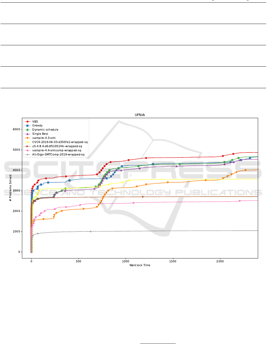
Table 2: The result table comparing 3 approaches to the Best solver and to best possible selector called VBS.

Benchmark: UFNIA AUFLIA QF NRA QF LIA

Best Solver

solver Vampire-4.3-smt Vampire-4.4 Yices 2.6.2 Z3-4.8.4

solved 4034 1382 2165 2946

PAR-2 13 189 767 1 242 230 3 307 748 1 005 170

VBS

solved 4875 1464 2659 3084

PAR-2 7 929 162 851 466 918 030 285 143

PAR-2 impr. ceiling 66.35 % 45.89 % 260.3 % 252.51 %

Single Best

solved 4510 1403 2498 3036

PAR-2 10 126 778 1 148 163 1 712 536 526 085

PAR-2 impr. 30.25 % 8.19 % 93.15 % 91.07 %

Greedy Schedule

solved 4655 1455 2582 3056

PAR-2 9 174 250 970 656 1302598 696 884

PAR-2 impr. 43.77 % 27.98 % 153.93 % 44.24 %

Dynamic Schedule

solved 4672 1431 2579 3049

PAR-2 9 501 057 1 020 999 1 320 703 481 244

PAR-2 impr. 38.82 % 21.67 % 150.45 % 108.87 %

Figure 3: Example result plot for UFNIA logic. It shows how many problems (y-axis) a given method solves up to a certain

time (x-axis). The greedy schedule performed best at the beginning. Schedules are different for each fold, but to get a better

idea here is an example of a greedy schedule for a single fold: ((z3-4.8.4, 1.83 s), (CVC4-2019-06-03, 125.5 s), (vampire-4.3,

2272.67 s)). In the end, the three methods achieved a similar number of solved examples.

4.3 Results

The results of three selected methods for four selected

benchmarks are summarized in table 2 and for UF-

NIA logic also shown in ﬁgure 3. The remaining ﬁg-

ures with graphs for other logics can be found in Ap-

pendix.

Our single best predictor based on interval predic-

tion performs very close to the EHM predictor in the

original MachSMT paper (we compare it to the PAR-

2 score for SolverLogic found on their Github

, al-

though direct comparison might be inaccurate since

the solver set could be different. Concretely, for

https://github.com/MachSMT/MachSMT/tree/

main/data/results/2019/SQ

Efﬁcient Solver Scheduling and Selection for Satisﬁability Modulo Theories (SMT) Problems

365

selected logics, they achieved: UFNIA: 10.58 %,

QF NRA: 92.27 %, AUFLIA: 12.44 % improvement

over best solver, for QF LIA we effectively removed

the best-performing solver SPASS-SAT in 2019 SQ

track so comparison does not make much sense. We

note that there is no signiﬁcant change in results with

different prediction regimes; one can predict directly

solving time, intervals as we do or even just classify

a problem in binary fashion to solved/unsolved (and

for an instance pick single best solver with the highest

probability for solving) while using the same predic-

tion model.

Overall, the greedy approach, which creates the

same schedule for all problems only by looking at

solving times and number of solved instances in the

training data, performed comparably or better than

other approaches. It is clear that this is caused by a

combination of long maximal runtime and fast solv-

ing times for solved instances. Selecting a single best

solver is easiest and would probably be the best op-

tion if the solving time was close to maximal runtime

on average. For example, in QF NRA some solvers

solved 75% of instances under 5s, and rarely did the

time needed to solve 75% of instances exceed 20s.

However, the greedy method is sensitive to the correct

time assignment for selected solvers. The dynamic

schedule worked pretty reliably on all benchmarks.

5 RELATED WORK

Algorithm selection and scheduling (Kadioglu et al.,

2011) is recognized as an important topic as a conse-

quence of the need for fast and reliable problem han-

dling in practical applications. Portfolio-based algo-

rithm selection with a machine learning model was

popularized by Leyton-Brown et al. (Leyton-Brown

et al., 2003).

The proposed work comes from MachSMT (Scott

et al., 2021), their main approach is to try to se-

lect only one solver from the whole portfolio. Ex-

cept EHM they also incorporate pairwise predictor

for solver selection. In the context of the selection of

logic solvers with EHM their predecessor is SATZilla

(Xu et al., 2008).

Our work is also related to various approaches that

use ML for solver scheduling, especially in the do-

main of SMT (Balunovic et al., 2018) use imitation

learning techniques to schedule strategies within the

Z3 solver. Similarly, (Ram

ırez et al., 2016) uses an

evolutionary algorithm to generate strategies for the

Z3 solver.

For an overview of various use cases of ML meth-

ods for combinatorial problems and algorithm selec-

tion, see the following survey papers: (Bengio et al.,

2020; Kerschke et al., 2019; Talbi, 2020). For a

more speciﬁc overview focused on GNNs, see (Cap-

part et al., 2021).

6 CONCLUSION

In conclusion, our research has introduced a novel ap-

proach to solving selection and scheduling that takes

advantage of dynamic scheduling policies and ma-

chine learning techniques. While our initial focus

was on the scheduling of Satisﬁability Modulo The-

ories (SMT) solvers, it is important to highlight that

our methodology extends beyond this speciﬁc appli-

cation. The selection and scheduling of algorithms is

widespread in various domains. Our work was not

intended solely to solve SMT solver scheduling, but

rather used scheduling of SMT solvers as a practical

example.

Our investigation revealed that the greedy sched-

ule, which does not rely on machine learning predic-

tions but instead selects solvers based on training data

statistics, often performed as well as or better than the

machine learning-based approach.

The results of this case study showed that solver

selection and scheduling are nuanced tasks and that

machine learning methods may not always offer clear

advantages over simpler approaches based on statis-

tics.

In future work, it would be valuable to further ex-

plore the dynamic scheduling approach, considering

its potential in scenarios where preemption and re-

sumption of solvers may be practically feasible.

ACKNOWLEDGEMENTS

The results were supported by the Ministry of Educa-

tion, Youth, and Sports within the dedicated program

ERC CZ under the project POSTMAN no. LL1902.

REFERENCES

Albawi, S., Mohammed, T. A., and Al-Zawi, S. (2017).

Understanding of a convolutional neural network. In

2017 international conference on engineering and

technology (ICET), pages 1–6. Ieee.

Amadini, R., Gabbrielli, M., and Mauro, J. (2014). Sunny:

a lazy portfolio approach for constraint solving. The-

ory and Practice of Logic Programming, 14(4-5):509–

524.

ICPRAM 2024 - 13th International Conference on Pattern Recognition Applications and Methods

366

Balunovic, M., Bielik, P., and Vechev, M. T. (2018). Learn-

ing to solve SMT formulas. In NeurIPS, pages 10338–

10349.

Barrett, C., Fontaine, P., and Tinelli, C. (2016). The

Satisﬁability Modulo Theories Library (SMT-LIB).

www.SMT-LIB.org.

Barrett, C., Stump, A., and Tinelli, C. (2010). The SMT-

LIB Standard: Version 2.0. In SMT Workshop.

Barrett, C. W., Conway, C. L., Deters, M., Hadarean, L.,

Jovanovic, D., King, T., Reynolds, A., and Tinelli, C.

(2011). CVC4. In Gopalakrishnan, G. and Qadeer,

S., editors, Computer Aided Veriﬁcation - 23rd In-

ternational Conference, CAV 2011, Snowbird, UT,

USA, July 14-20, 2011. Proceedings, volume 6806 of

Lecture Notes in Computer Science, pages 171–177.

Springer.

Bengio, Y., Lodi, A., and Prouvost, A. (2020). Machine

learning for combinatorial optimization: a method-

ological tour d’horizon. European Journal of Oper-

ational Research.

Bjørner, N. and de Moura, L. (2014). Applications of smt

solvers to program veriﬁcation. Notes for the Summer

School on Formal Techniques.

Bruttomesso, R., Cimatti, A., Franz

en, A., Griggio, A.,

and Sebastiani, R. (2008). The mathsat 4 smt solver:

Tool paper. In Computer Aided Veriﬁcation: 20th

International Conference, CAV 2008 Princeton, NJ,

USA, July 7-14, 2008 Proceedings 20, pages 299–303.

Springer.

Cappart, Q., Ch

etelat, D., Khalil, E., Lodi, A., Morris, C.,

and Veli

ckovi

c, P. (2021). Combinatorial optimiza-

tion and reasoning with graph neural networks. arXiv

preprint arXiv:2102.09544.

Crouse, M., Abdelaziz, I., Cornelio, C., Thost, V., Wu,

L., Forbus, K., and Fokoue, A. (2019). Improv-

ing graph neural network representations of logi-

cal formulae with subgraph pooling. arXiv preprint

arXiv:1911.06904.

De Moura, L. and Bjørner, N. (2008). Z3: An efﬁcient smt

solver. In International conference on Tools and Algo-

rithms for the Construction and Analysis of Systems,

pages 337–340. Springer.

de Moura, L. and Bjørner, N. (2012). Applications and chal-

lenges in satisﬁability modulo theories. In Workshop

on Invariant Generation (WING), volume 1, pages 1–

11. EasyChair.

Dutertre, B. (2014). Yices 2.2. In International Confer-

ence on Computer Aided Veriﬁcation, pages 737–744.

Springer.

Erickson, N., Mueller, J., Shirkov, A., Zhang, H., Larroy,

P., Li, M., and Smola, A. (2020). Autogluon-tabular:

Robust and accurate automl for structured data. arXiv

preprint arXiv:2003.06505.

Glorot, X., Anand, A., Aygun, E., Mourad, S., Kohli, P., and

Precup, D. (2019). Learning representations of logi-

cal formulae using graph neural networks. In Neural

Information Processing Systems, Workshop on Graph

Representation Learning.

Godefroid, P., Levin, M. Y., and Molnar, D. A. (2012).

SAGE: whitebox fuzzing for security testing. Com-

mun. ACM, 55(3):40–44.

Hamilton, W. L. (2020). Graph representation learning.

Synthesis Lectures on Artiﬁcial Intelligence and Ma-

chine Learning, 14:1–159.

ula, J., Moj

sek, D., and Janota, M. (2021). Graph neural

networks for scheduling of smt solvers. In 2021 IEEE

33rd International Conference on Tools with Artiﬁcial

Intelligence (ICTAI), pages 447–451. IEEE.

Kadioglu, S., Malitsky, Y., Sabharwal, A., Samulowitz, H.,

and Sellmann, M. (2011). Algorithm selection and

scheduling. In International Conference on Principles

and Practice of Constraint Programming.

Ke, G., Meng, Q., Finley, T., Wang, T., Chen, W., Ma, W.,

Ye, Q., and Liu, T.-Y. (2017). Lightgbm: A highly

efﬁcient gradient boosting decision tree. Advances in

neural information processing systems, 30.

Kerschke, P., Hoos, H. H., Neumann, F., and Trautmann, H.

(2019). Automated algorithm selection: Survey and

perspectives. Evolutionary computation, 27(1):3–45.

Leyton-Brown, K., Nudelman, E., Andrew, G., McFadden,

J., and Shoham, Y. (2003). A portfolio approach to

algorithm selection. In IJCAI, volume 3, pages 1542–

1543.

Leyton-Brown, K., Nudelman, E., and Shoham, Y. (2009).

Empirical hardness models: Methodology and a case

study on combinatorial auctions. Journal of the ACM

(JACM), 56(4):1–52.

Pimpalkhare, N. (2020). Dynamic algorithm selection for

SMT. In 2020 35th IEEE/ACM International Con-

ference on Automated Software Engineering (ASE),

pages 1376–1378. IEEE.

Ram

ırez, N. G., Hamadi, Y., Monfroy,

E., and Saubion, F.

(2016). Evolving SMT strategies. In ICTAI.

Scott, J., Niemetz, A., Preiner, M., Nejati, S., and Ganesh,

V. (2021). Machsmt: A machine learning-based algo-

rithm selector for smt solvers. In International Con-

ference on Tools and Algorithms for the Construction

and Analysis of Systems, pages 303–325. Springer.

Selvaraju, R. R., Cogswell, M., Das, A., Vedantam, R.,

Parikh, D., and Batra, D. (2017). Grad-cam: Visual

explanations from deep networks via gradient-based

localization. In Proceedings of the IEEE international

conference on computer vision, pages 618–626.

Talbi, E.-G. (2020). Machine learning into metaheuristics:

A survey and taxonomy of data-driven metaheuristics.

ACM Computing Surveys.

Wang, M., Tang, Y., Wang, J., and Deng, J. (2017). Premise

selection for theorem proving by deep graph embed-

ding. In NeurIPS.

Xu, L., Hutter, F., Hoos, H. H., and Leyton-Brown, K.

(2008). Satzilla: portfolio-based algorithm selection

for sat. Journal of artiﬁcial intelligence research,

32:565–606.

Zhao, W., Ramamritham, K., and Stankovic, J. A.

(1987). Preemptive scheduling under time and re-

source constraints. IEEE Transactions on computers,

100(8):949–960.

Efﬁcient Solver Scheduling and Selection for Satisﬁability Modulo Theories (SMT) Problems

367

APPENDIX

Additional Graphs and Dynamic

Schedule Algorithm

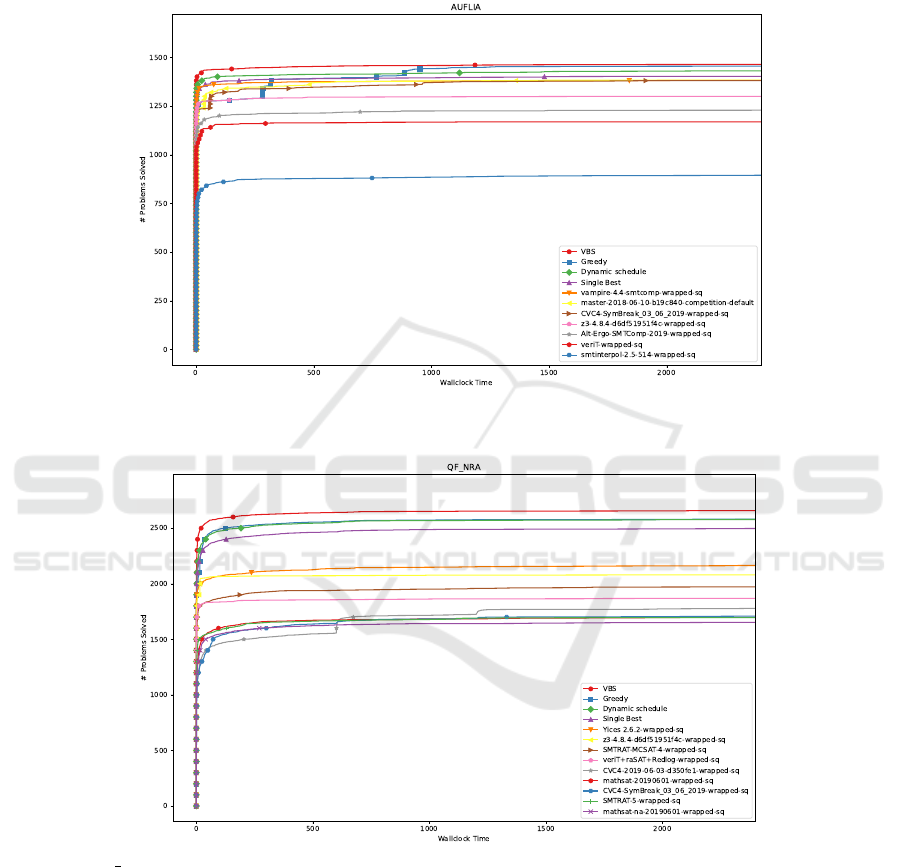
Figure 4: On AUFLIA greedy method solved almost the same number instances as VBS. The drawback is that at the beginning

of runtime it did not perform as well.

Figure 5: In QF NRA logic the dynamic schedule performed very similarly to the greedy one, while both outperformed single

solver selection by considerable amount.

ICPRAM 2024 - 13th International Conference on Pattern Recognition Applications and Methods

368

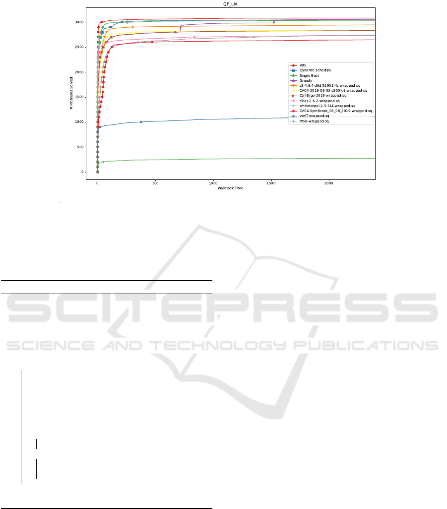
Figure 6: In QF LIA the greedy schedule did not perform as well as others. The reason behind it is that the average solving

times for selected solvers in training data were very small, and at the same time very similar, thus applying the greedy method

in the same way as to other logics, split the runtime between the selected 3 solvers evenly (two visible jumps in number of

solved instances). This shows that our greedy method cannot be applied blindly and one should consider a different way

of solving time assignment. Greedy schedule example from a single fold: ((Ctrl-Ergo-2019, 713.77 s), (CVC4-2019-06-03,

808.76 s), (z3-4.8.4, 877.45 s)), although 75% of the solved examples in the entire dataset are solved by 12.9 s, 18.88 s and

18.42 s by these solvers, respectively.

Algorithm 1: Dynamic scheduling with predictions.

Data: D: array of lists. List

D[i] = [(t

, d

), . . . , (t

, d

)] corresponds to

solver i with t

being the length of the j-th

interval and d

its score.

Result: Total runtime spent on the formula

1 runtime ← 0;

2 while runtime < timeout do

3 expectedTimes ← getExpectedTimes(D) ;

4 currBest ← argmin(expectedTimes);

5 nextIntLen, score ← getFirst(D[currBest]);

6 solved, time ←

runSolver(currBest, nextIntLen);

7 runtime ← runtime + time;

8 if solved then

9 return runtime;

10 else

11 D[currBest] ←

removeFirst(D[currBest]);

12 return 2 × timeout; // unsolved instance

penalty

Efﬁcient Solver Scheduling and Selection for Satisﬁability Modulo Theories (SMT) Problems

369