Modeling Batch Tasks Using Recurrent Neural Networks in Co-Located

Alibaba Workloads

Hifza Khalid

1 a

, Arunselvan Ramaswamy

2 b

, Simone Ferlin

3 c

and Alva Couch

1 d

Department of Computer Science, Tufts University, MA, U.S.A.

Karlstad University, Sweden

Red Hat and Karlstad University, Sweden

Keywords:

Cloud Workload Modeling, Co-Located Workloads, Time Series Forecasting, Recurrent Neural Networks.

Abstract:

Accurate predictive models for cloud workloads can be helpful in improving task scheduling, capacity plan-

ning and preemptive resource conﬂict resolution, especially in the setting of co-located jobs. Alibaba, one of

the leading cloud providers co-locates transient batch tasks and high priority latency sensitive online jobs on

the same cluster. In this paper, we consider the problem of using a publicly released dataset by Alibaba to

model the batch tasks that are often overlooked compared to online services. The dataset contains the arrivals

and resource requirements (CPU, memory, etc.) for both batch and online tasks. Our trained model predicts,

with high accuracy, the number of batch tasks that arrive in any 30 minute window, their associated CPU and

memory requirements, and their lifetimes. It captures over 94% of arrivals in each 30 minute window within a

95% prediction interval. The F1 scores for the most frequent CPU classes exceed 75%, and our memory and

lifetime predictions incur less than 1% test data loss. The prediction accuracy of the lifetime of a batch-task

drops when the model uses both CPU and memory information, as opposed to only using memory informa-

tion.

1 INTRODUCTION

Businesses today are routinely required to perform

resource-intensive computations but often lack suf-

ﬁcient on-site resources. As a consequence, many

computational jobs are ofﬂoaded to the “cloud”. The

cloud refers to off-site resources that may be accessed

via the Internet. Such cloud services run on shared

clusters within data centers to lower costs and im-

prove resource utilization (Zhang et al., 2022). There-

fore, jobs from different parties are co-located on the

same machines. While co-location improves machine

utilization, it poses a number of challenges to the data

center, including security (isolation between different

services), scheduling and performance interference

(Jiang et al., 2022), (Xu et al., 2018). Additionally,

different jobs or services may contend for the same

resources causing service delays that affect Quality of

Service (QoS) of applications (Chen et al., 2018).

https://orcid.org/0000-0003-2929-0454

https://orcid.org/0000-0001-7547-8111

https://orcid.org/0000-0002-0722-2656

https://orcid.org/0000-0002-4169-1077

To address these challenges and improve cloud

operation, efﬁcient planning and optimization is re-

quired (Grandl et al., 2014). For example, through

better planning of which resources to provision and

when, capacity planners can proactively support fu-

ture workloads while trying to avoid resource short-

age and contention issues (Bergsma et al., 2021).

Contention can negatively effect performance and ef-

ﬁciency of co-located workloads. It leads to increased

pressure on memory resources due to increased pag-

ing and swapping activities, all of which ultimately

lead to QoS degradation and unpredictable applica-

tion behavior. By understanding the properties and

behavior of co-located workloads from real produc-

tion environments, we can improve decision making

in the cloud. (Liu and Yu, 2018) characterized a trace

of co-located workloads from Alibaba’s production

cluster to study some of these properties like the het-

erogeneity of clouds. We, on the other hand, propose

the development of a workload prediction model to

provide better estimates of future workloads for im-

proved scheduling and capacity planning decisions.

Accurate cloud workload models are valuable for

improved decision-making and planning within cloud

558

Khalid, H., Ramaswamy, A., Ferlin, S. and Couch, A.

Modeling Batch Tasks Using Recurrent Neural Networks in Co-Located Alibaba Workloads.

DOI: 10.5220/0012392700003654

Paper published under CC license (CC BY-NC-ND 4.0)

In Proceedings of the 13th International Conference on Pattern Recognition Applications and Methods (ICPRAM 2024), pages 558-569

ISBN: 978-989-758-684-2; ISSN: 2184-4313

management systems. However, the task of accu-

rately modeling these workloads is inherently chal-

lenging due to the “heterogeneous” and “imbalanced”

nature of the cloud with respect to resource alloca-

tion and lifespan (Verma et al., 2014). Modeling co-

located jobs presents an even greater challenge due

to additional factors such as interference, resource

contention, complex inter-job dependencies, varying

resource demands and isolation requirements, all of

which render simplistic modeling techniques inade-

quate.

Addressing this gap, this paper proposes a Ma-

chine Learning (ML) based approach to workload

modeling using real-world cloud data. While this

method is expected to be accurate and realistic, the

availability of such data is a challenge. Cloud

providers are generally reluctant to publicly release

their data (Calzarossa et al., 2016). Even when data is

available, it is often limited, making it challenging for

reliable training of ML algorithms. In this paper, we

work with one such dataset from Alibaba (Alibaba,

2018). A workload model derived from such a dataset

can not only be used for better planning decisions

in cloud environments, but also for generating real-

istic synthetic workloads, which, in turn, can proac-

tively support tuning systems without large downtime

or data gathering (Bergsma et al., 2021).

The Alibaba dataset considered in this work con-

sists of traces of co-located workloads over an eight

day period (Alibaba, 2018). It consists of online

services and batch workloads. We focus on model-

ing batch workloads as online services are guaran-

teed resources due to their high priority, while batch

jobs are executed on the remaining resources left on

the servers. By modeling batch workloads, we hope

that it can lead to their improved resource utilization,

performance and efﬁciency. Batch jobs in Alibaba’s

dataset are divided into tasks, where task executions

are subject to dependency constraints. These tasks are

further divided into instances that have the same bi-

nary code and resource requests but different input

data. We model batch tasks in our work as they are

the smallest unit of batch jobs for which we have in-

formation about resource requirements and comple-

tion times. This low-level model can be readily used

to model batch jobs if needed.

Our model, explained in Figure 2, uses the

Alibaba dataset to predict arrivals, associated re-

source requirements, and lifetimes/completion times

for batch tasks. To model arrivals, we use the Autore-

gressive Integrated Moving Average (ARIMA) model

(E. P. Box et al., 1970). ARIMA is a popular time

series forecasting model that has the ability to cap-

ture trends and seasonality. To model the resources

requirements and completion times, we use a Long

Short-term Memory (LSTM) based neural network

as such networks can capture long-term dependen-

cies (Siami-Namini et al., 2018). Our model can

reproduce the Alibaba dataset with very high accu-

racy. In order to be fully practical, our model must

be able to generate random yet realistic workloads.

This can be very easily realized by tuning parameters

of the ARIMA model or by modeling the probability

distributions over the resource requirements and life-

time through the use of Bayesian Machine Learning

methods such as Gaussian Process Regression. Addi-

tionally, we can model arrivals as a Poisson process,

an approach adopted in (Bergsma et al., 2021) when

modeling Virtual Machine (VM) arrivals in Microsoft

Azure (Cortez et al., 2017).

The remaining sections of the paper are organized

as follows: Section 2 discusses background and re-

lated research; Section 3 describes the Alibaba dataset

and our approach to model the batch tasks; Section 4

explains the setup used for training models; Section 5

presents the results from the experiments; and ﬁnally,

Section 6 concludes the paper.

2 BACKGROUND AND RELATED

WORK

Bergsma et al. (Bergsma et al., 2021) modeled the

production virtual machine workload from two real-

world cloud providers, Microsoft and Huawei, and

demonstrated its applications in scheduling and ca-

pacity planning. While we found their work inspir-

ing, it did not account for co-located workloads. Co-

located workloads have become increasingly preva-

lent in modern cloud environments, with leading

cloud providers like Google and Alibaba adopting the

technique to enhance cost efﬁciency and optimize re-

source utilization (Tirmazi et al., 2020). Costa et al.

(Da Costa et al., 2018) modeled Google’s co-located

traces using statistical methods and clustering tech-

niques, however, their work does not address our spe-

ciﬁc problem. Google’s cluster management system

operates on a monolithic architecture, utilizing a cen-

tralized resource scheduler for resource allocation and

management (Cheng et al., 2018), whereas our focus

is on online and batch services managed by separate

schedulers. Moreover, Google’s dataset does not con-

tain workload (online and batch) speciﬁc information,

making it challenging to characterize different work-

loads when co-located.

Acquiring realistic workload data for modeling is

challenging as most cloud providers, apart from a few

exceptions such as Google (Reiss et al., 2011), Al-

Modeling Batch Tasks Using Recurrent Neural Networks in Co-Located Alibaba Workloads

559

ibaba (Alibaba, 2018), and Microsoft (Cortez et al.,

2017), are reluctant to disclose their data. Addi-

tionally, scholarly papers rarely provide information

about their data collection methods or even release it

for reproducibility. For this reason, we selected Al-

ibaba’s publicly available dataset, which offers dis-

tinct information for batch and online services, en-

abling us to delve deeper into the characteristics of

co-located workloads.

Within the Alibaba dataset, we opted to initially

focus on modeling batch services. This choice stems

from the observation that batch services generally uti-

lize more CPU resources than online services (Liu

and Yu, 2018). Furthermore, due to the prioritization

of online services, they are executed within containers

that receive a dedicated allocation of resources, leav-

ing only a limited set of resources available for batch

services. This allocation strategy ensures the avail-

ability of resources for online services at all times.

Therefore, by gaining insights into batch workloads,

we aim to enhance job scheduling for batch services

and optimize resource provisioning for co-located

workloads. To the best of our knowledge, we have not

come across any existing work focused on modeling

co-located workloads or exclusively batch services.

We now brieﬂy discuss some of the past research

in cloud workload modeling. Moreno et al. (Moreno

et al., 2014) have previously modeled arrival rates,

resource requirements, and job duration for speciﬁc

users in a Google cloud trace. In contrast, our ap-

proach does not rely on user-speciﬁc information, al-

lowing us to apply it more broadly to model large-

scale future workloads. Similarly, a workload gen-

erator is presented by Bahga and Madisetti (Bahga

et al., 2011) to evaluate cloud applications. They sim-

ulate user behavior with inter-session times and ses-

sion duration. A number of papers focus solely on

modeling job arrival rates (Juan et al., 2014), (Koltuk

and Schmidt, 2020), whereas our work models task

arrivals, resource requirements, and task completion

times within batch services. In addition, there has

been a lot more work on VM scheduling/co-location

rather than workloads in clusters (Cortez et al., 2017),

where the challenges as well as the solutions are not

necessarily applicable to our problem.

One of the most popular stochastic models in time

series forecasting is the ARIMA model developed by

Box and Jenkin (E. P. Box et al., 1970). It can capture

noise, trend as well as the seasonal component in the

dataset (Herbst et al., 2013). Rodrigo et al. (Calheiros

et al., 2015) used it to successfully predict hourly web

requests to English Wikipedia resources. Due to its

simplicity and ﬂexibility, it has also been used to pre-

dict cloud coverage (weather) (Yu Wang and Xiao,

2018), tourist arrivals (Ching-Fu Chen and Chang,

2009) and short-term resource usage in the cloud (Ja-

nardhanan and Barrett, 2017) with high accuracy. We

used it to model the batch-task arrival counts in our

dataset. To model the resource requirements and life-

times, we used LSTM, a type of recurrent neural net-

work which excels at capturing long-term dependen-

cies. It has been used to model VM resource require-

ments and lifetime in the Microsoft dataset (Cortez

et al., 2017) by Shane et al (Bergsma et al., 2021).

3 OUR APPROACH

Alibaba dataset contains more than 14 million data

points. It captures co-located online and batch jobs

from a cluster of 4034 machines over an eight-day pe-

riod. The dataset is described in detail below.

3.1 Alibaba Dataset and Batch Task

Modeling

Alibaba’s cluster management system oversees re-

sources for two different kinds of workloads: online

and batch. It comprises of two different schedulers,

namely Sigma and Fuxi, each of which operates with

its own dedicated resource pool. Sigma is responsi-

ble for user-facing, long-running online services ex-

ecuted within containers, while Fuxi handles batch

jobs executed directly on physical hosts as shown in

Figure 1. To facilitate improved scheduling deci-

sions, Sigma and Fuxi share cluster state information.

The dataset collected from this system contains in-

formation about server metadata, server usage, con-

tainer metadata, container usage, and batch tasks and

batch instances. More speciﬁcally, the data contains

information about status, resource usage, resource re-

quirements, arrival and completion times of submitted

jobs.

Batch-processing applications utilize predeﬁned

limited amount of resources, with a low priority. In

cases with insufﬁcient resources for a newly arrived

online job, some or all of the batch jobs are preempted

to free-up resources. While batch jobs are not latency

critical, preempting them leads to overhead involved

in rescheduling. To avoid rescheduling, batch work-

loads are typically scheduled in windows when the

arrival rate of online jobs is lower, e.g, typically, late

at night. Such policies clearly give latency-critical

applications preference over batch-processing appli-

cations (Guo et al., 2019). Modeling these processes

(both online and batch jobs) is imperative for better

analysis and better utilization of available resources.

In this paper, we focus on modeling batch jobs.

ICPRAM 2024 - 13th International Conference on Pattern Recognition Applications and Methods

560

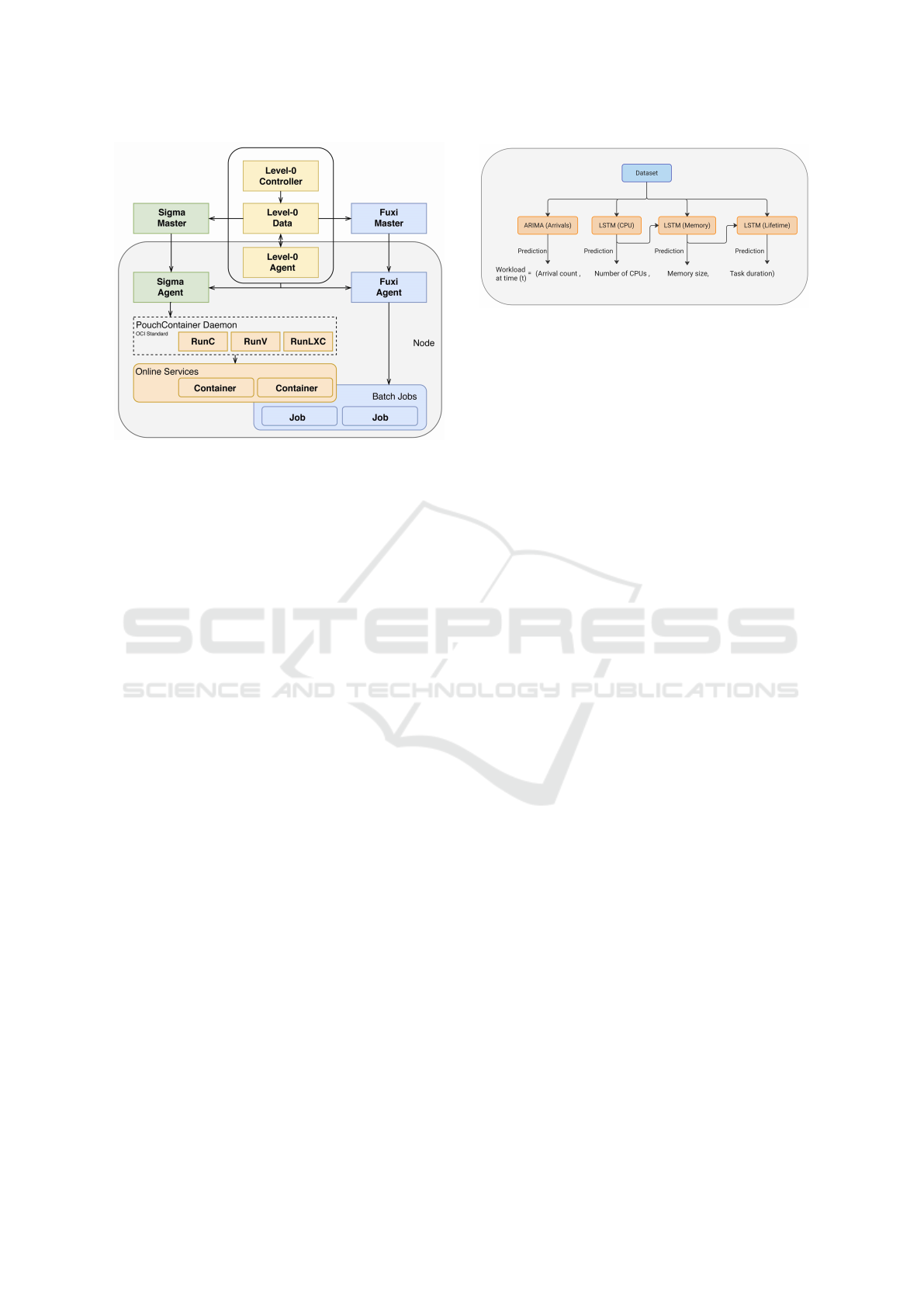
Figure 1: The architecture of Alibaba cluster management

system (Alibaba, 2018).

Let us now take a closer look at batch jobs. Each

batch job consists of one or more tasks. These tasks

can have dependencies, where the completion of one

task predicates the completion of others. This inter-

dependence can be represented as a directed acyclic

graph. Further, each task may create one or more in-

stances with the same binary code and resource re-

quests but with different input data. Such an instance

is the basic scheduling unit in Alibaba Cluster Man-

agement System. The duration of a job is the sum of

its task durations. The duration of a task is the sum of

the execution time of all its instances. More specif-

ically, the Alibaba dataset contains the following in-

formation with respect to the tasks (from some batch

job):

1. Start and End times.

2. Requested CPU and memory resources

3.2 Workload Prediction Model

Figure 2 illustrates our workload prediction model.

Using the Alibaba dataset from Section 3.1, this

model predicts the following:

1. The number of batch tasks that arrive within the

30 minute window.

2. The number of CPU, memory requirements for

each arrival within the t

30 minute window.

3. The lifetime of each arrival within the t

minute window.

The dataset is used to train four different ML mod-

els. Speciﬁcally, the Autoregressive Integrated Mov-

ing Average (ARIMA) model is trained to forecast ar-

rival counts, while three Long Short-Term Memory

Figure 2: Illustration of the Workload Prediction Model.

(LSTM) networks are trained to predict the CPU and

memory requirements as well as lifetimes. In order to

predict memory requirements, we use the predicted

CPU requirements as input. Conversely, for the life-

time model, we use memory requirements as input.

In Section 4, we delve into the qualitative impact of

using CPU requirements to predict memory and mem-

ory to predict lifetimes. Now, we provide an overview

of ARIMA and LSTM networks, along with an expla-

nation for our choice of these models.

3.2.1 ARIMA for Arrivals

In the statistical parlance, the sequence of arrival

counts within successive 30 minute windows consti-

tutes a non-stationary time series data. This data may

exhibit variations, such as higher workload arrivals

during the day compared to night. This trend may

vary across days of the week, e.g., the weekends may

be quieter. The ARIMA model is a popular statistical

method that is often used to ﬁt non-stationary time se-

ries data. It can also account for seasonal patterns in

the data. In summary, the ARIMA model has three

key components:

• “AR” (Autoregressive). This component ac-

counts for temporal dependencies by regressing

over the past values of the evolving variable - ar-

rival counts in our case.

• “I” (Integrated). It involves differencing the data

to achieve stationarity, enabling more accurate

predictions.

• “MA” (Moving Average). This component con-

siders moving averages to capture the average

changes in values, which helps in understanding

the evolving patterns of arrival counts over time.

These three components are deﬁned by the pri-

mary model parameters: p, d and q, for the non-

seasonal aspects of the data, and P, D, Q for their

seasonal counterparts. Additionally, the model can

be parameterized by the number of periods within

every season, denoted as s. It is trained using the

Box-Jenkins method (E. P. Box et al., 1970), (Siami-

Namini et al., 2018). Recall that the Alibaba dataset

Modeling Batch Tasks Using Recurrent Neural Networks in Co-Located Alibaba Workloads

561

contains the start times for batch tasks over an eight

day period. As a preprocessing step, these start times

are used to generate the time series dataset that is the

number of arrivals within each 30-minute window.

The ARIMA model is trained using this transformed

dataset for prediction and analysis. The dataset is di-

vided into 30-minute intervals, as using shorter inter-

vals would result in longer seasonal periods, which

can pose challenges for ARIMA modeling (Hynd-

man, 2010).

3.2.2 LSTM for CPU, Memory and Lifetimes

We used LSTM networks to predict the CPU and

memory requirements, and the lifetime of a batch

task. Unlike a regular feedforward network, LSTMs

are artiﬁcial neural networks capable of processing

feedback. They are composed of special long short-

term memory units designed to capture temporal in-

formation effectively. LSTMs are particularly well-

suited for time series forecasting applications, espe-

cially when datasets contain relevant events separated

in time. In the Alibaba dataset, the task executions are

governed by a dependency graph. Speciﬁcally, a task

may only be executed provided a previous task has

already been executed. When predicting the resource

requirements (CPU, memory) or lifetime, it is impor-

tant to consider other related tasks that have been sub-

mitted for execution.

Alibaba dataset features 16 distinct CPU and over

300 unique memory values. To address these differ-

ent prediction tasks, we use two separate LSTMs. In

particular, we train the CPU-LSTM as a 16-class clas-

siﬁer whereas the memory-LSTM is trained using re-

gression. Additionally, we include CPU requirement

as an input feature when predicting memory. How-

ever, our ﬁndings in Section 4 show that the inclusion

of CPU does not signiﬁcantly enhance the accuracy

of memory predictions. In other words, memory can

be predicted accurately without explicitly considering

CPU. Lastly, we consider the problem of predicting

task lifetimes. In the dataset, each task is associated

with one of four states: terminated, running, waiting

or failed. Our analysis focuses exclusively on predict-

ing successfully terminated tasks, which account for

over 98% of the dataset. As in the case of memory,

we employ an LSTM model trained through regres-

sion to predict the lifetime of a task. The LSTM takes

the (predicted) memory requirement as an additional

input. We also conducted experiments wherein we

used both CPU and memory as input. However, we

found that the prediction accuracy is better when the

input is memory alone.

4 EXPERIMENTAL SETUP

In order to present our numerical results, we need to

ﬁrst specify the setup used to conduct the various ex-

periments. We begin by noting that we used Python

3.10 for all our experiments. Our models are ML

based, and Python provides the best libraries to im-

plement them.

4.1 Data Preprocessing

Since we predict the number of batch arrivals in a

given 30-minute window, we begin by preprocessing

the dataset to generate time series data containing task

arrival counts in consecutive 30-minute windows. As

each task is associated with a start and an end time,

this preprocessing step is fairly straightforward. We

use ARIMA to ﬁt the resulting time series data. We

use Python’s pmdarima package, and call on the func-

tion auto-arima for training on the arrival count time

series. The CPU and memory requirements, and the

completion times are ﬁtted using LSTM networks. As

there are only 16 unique values for CPU, we solve

the CPU prediction as a classiﬁcation problem. For

memory and lifetime predictions, we adopt a regres-

sion approach. We use keras API, which is devel-

oped by Google and is a popular choice to train neu-

ral networks, to train our LSTMs. In the next section,

we discuss the various hyperparameters involved in

training.

4.2 Modeling Hyperparameters

We begin by noting the hyperparameters for the sea-

sonal ARIMA model. While in traditional ARIMA

models, p, d, and q values needed to be speciﬁed,

Seasonal ARIMA (SARIMA) models require, in ad-

dition, the speciﬁcation of seasonal parameters P, D,

Q, and s. The parameter s represents the length of the

seasonal period, which varies depending on the recur-

rent periodicity in the data. For instance, a daily peri-

odicity corresponds to a value of 7, while weekly and

monthly periodicities have values of 52 and 12, re-

spectively. In our case, we are modeling day-over-day

seasonality in an 8-day dataset, with arrival counts

aggregated over 30-minute periods each day. There-

fore, the value of s is set to 48, which corresponds

to the number of 30-minute buckets in a 24-hour day.

The ARIMA hyperparameters are tuned using the Al-

ibaba dataset to increase prediction accuracy by the

auto-arima function. The recommended model uses

p = 4, d = 0, q = 3 in the non-seasonal part and P = 2,

D = 0 and Q = 1 to model the non-seasonal compo-

nents of the data.

ICPRAM 2024 - 13th International Conference on Pattern Recognition Applications and Methods

562

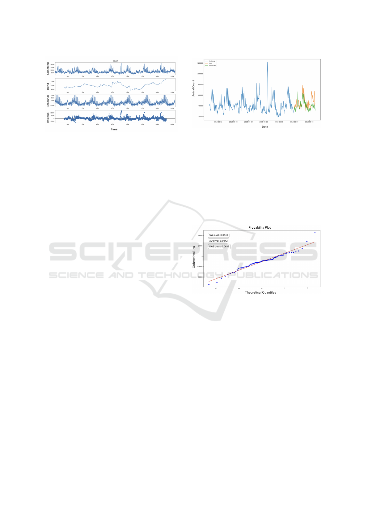
Figure 3: Time series decomposition of arrival counts.

Now, we look at the hyperparameters tuned for the

LSTMs used to predict the resources and the lifetime.

We use the same LSTM network for the three pre-

diction tasks. In particular, all our LSTMs are sin-

gle layered with 32 hidden LSTM activations. The

classiﬁcation-LSTM uses a soft-max output layer,

while the other two LSTMs use a linear output layer.

Since LSTMs are trained using the Back-Propagation

Through Time (BPTT) algorithm, we need to spec-

ify the number of steps in time that the BPTT al-

gorithm must look back. Our models look 10 steps

back in time. The optimizer used is the Stochastic

Gradient Descent (SGD) with momentum algorithm.

We use a decaying learning rate starting from 0.001

and a momentum value of 0.9. The learning rate de-

cays as a function of the epochs. When it comes to

the loss functions, the classiﬁcation problem uses the

cross-entropy loss, and the regression problems use

the mean-squared loss.

5 EXPERIMENTAL RESULTS

We present the results from various experiments in

this section. We start by looking at the task arrivals

prediction model.

5.1 ARIMA - Arrivals

It is essential to eliminate non-stationarities in data

for ARIMA to have a high prediction accuracy. There

is an “initial differencing” step in ARIMA that is

repeated a few times in order to eliminate non-

stationarities. The number of repetitions are deter-

mined by the parameter d. In order to ﬁnd the optimal

d, we used the Augmented Dickey-Fuller (ADF) sta-

tistical test (Fattah et al., 2018). The general guideline

for the ADF test is that if the p-value is less than the

critical value of 0.05, the d differencing steps have

eliminated trends. In our case, for the chosen d pa-

rameter value of 1, the p-value was 4.5e − 07 which

is less than 0.05.

Figure 4: Prediction results for ARIMA model.

All time series data have four components: av-

erage value, trend (i.e. an increasing or decreasing

mean), seasonality (i.e. a repeating cyclical pattern),

and residual (random noise) (Mitrani, 2020). Trends

and seasonality are not always present in time depen-

dent data, so we performed decomposition to identify

any underlying seasonal patterns. Figure 3 illustrates

the decomposition of the arrival counts data, where

it clearly displays daily seasonality. As a result of

this analysis, we decided to use SARIMA instead of

ARIMA to model arrival counts.

Figure 5: Probability-to-Probability (PP) Plot and Normal-

ity Tests for prediction errors in ARIMA model.

Figure 4 shows the modeling results for the num-

ber of task arrivals per 30-minute time intervals us-

ing SARIMA. The model uses 70% of the data for

training and 30% for testing. As shown, the predicted

values effectively capture seasonality as well as the

bursts in the data.

We use prediction intervals to evaluate our

model using Root Mean Squared Forecasting Er-

ror (RMSFE) (Brownlee, 2020). The valid-

ity of this approach relies on the assumption that

the residuals of our validation (or test) predictions

are normally distributed. To test this assumption,

we used a Probability-to-Probability (PP) plot, and

tested the normality of our prediction errors us-

ing the Anderson-Darling, Kolmogorov-Smirnov, and

D’Agostino K-squared (Mishra, 2020) tests. The PP-

plot compares the data sample with the plot of a nor-

mal distribution. Ideally, when the data follows a

Modeling Batch Tasks Using Recurrent Neural Networks in Co-Located Alibaba Workloads

563

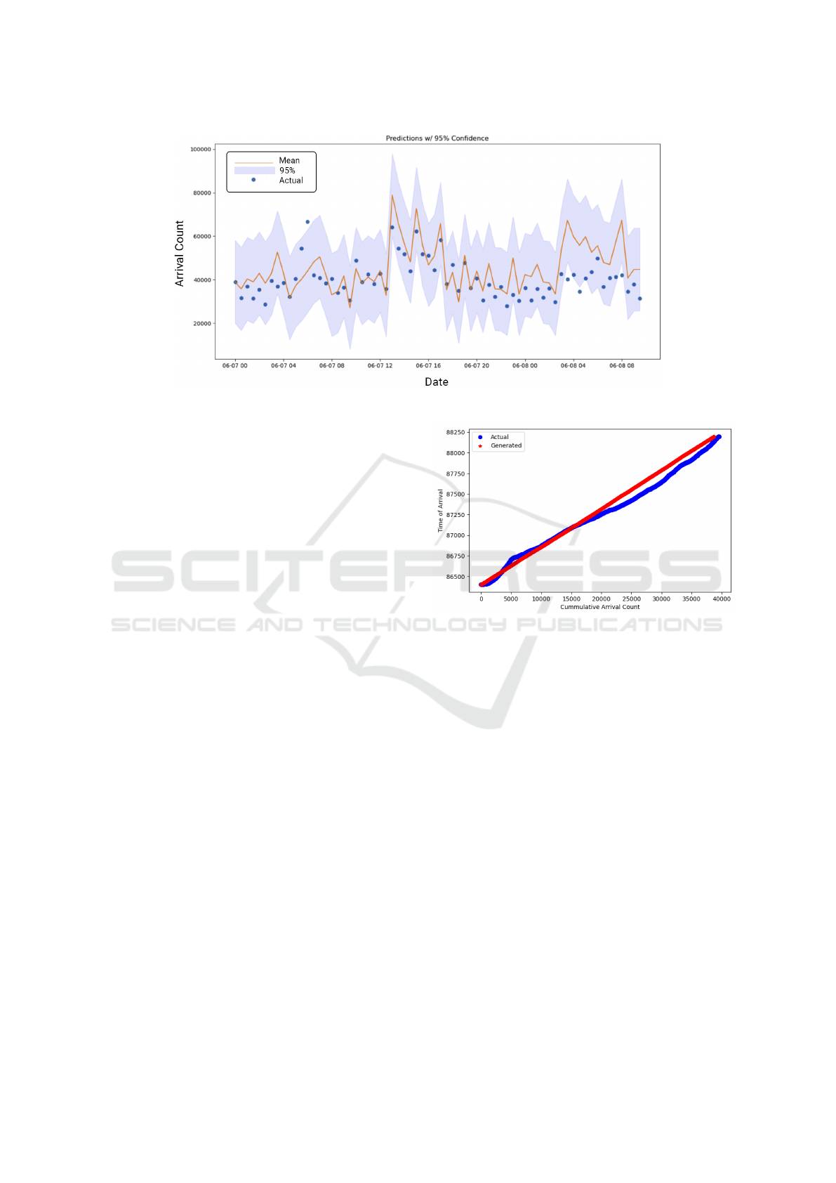
Figure 6: Actual and generated (with mean and 95% prediction intervals) arrival counts.

normal distribution, the data points align to form a

straight line. The three normality tests use p-values

to determine how likely it is that a data comes from a

population that follows a normal distribution. If the p-

values for all tests are greater than a chosen α thresh-

old, there is evidence to suggest that the data comes

from a normal distribution. Figure 5 shows that all

three tests returned a p-value larger than the α = 0.01,

therefore, indicating that our data points come from a

normal distribution.

We used a prediction interval of 95% to evaluate

our model. In a normal distribution, approximately

95% of the data points lie within 1.96 standard devia-

tions of the mean. Hence, to determine the size of our

prediction interval, we multiplied 1.96 by the RMSFE

for our arrival counts model. The results, as shown in

Figure 6, indicate that our model captures over 94%

of the data points within the 95% prediction interval.

The line in the ﬁgure represents the mean of predic-

tions. Another noteworthy aspect of our model is that

it tends to slightly overestimate the arrivals in approx-

imately 90% of the cases. This indicates that while

our model can be utilized for an informed planning

of the future through forecasting, it also exhibits the

ability to accommodate small estimation errors and

operate under small variations in expected load.

We modeled individual arrivals within each 30-

minute period by a Poisson process. Since a ran-

domly distributed set of arrival times will have sub-

sequent times exponentially-distributed, we modeled

individual arrivals in any given 30-minute period by

sampling its arrival count from a uniform distribution.

The actual and generated results for one time period

are shown in Figure 7.

Figure 7: Actual and generated individual arrivals over one

time period.

5.2 LSTM - CPU, Memory, Lifetime

As stated earlier, we model both resource require-

ments and task lifetime in our dataset using LSTMs.

Note that the resource requirements include both CPU

and memory resources.

5.2.1 CPU

Considering that our dataset consists of over 14 mil-

lion data points with only 16 unique values for CPU,

we opted for a classiﬁcation approach to model CPU.

The dataset was divided into three subsets: training,

validation, and testing, with 75% of the data allo-

cated for training and validation, and the remaining

25% for testing. The input data was one-hot encoded

before feeding it to LSTM. To train our model, we

used time series cross validation with k = 10. Our

LSTM comprised of a single layer with 32 hidden

nodes and used the SGD optimizer with a decaying

learning rate of 0.001. The loss was calculated us-

ing the ‘cross-entropy’ function. The cross-entropy

ICPRAM 2024 - 13th International Conference on Pattern Recognition Applications and Methods

564

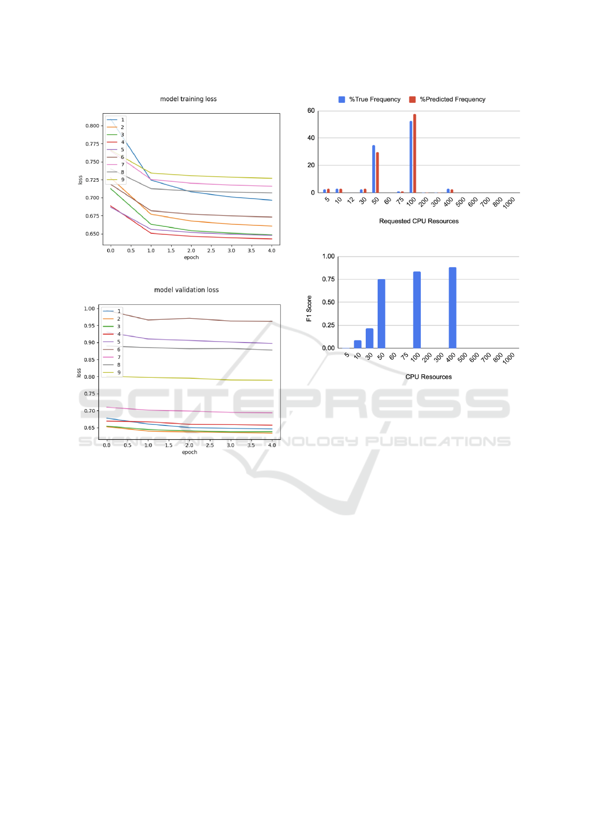
Figure 8: Cross entropy training loss for CPU.

Figure 9: Cross entropy validation loss for CPU.

for different epochs and time series cross-validation

splits for the training and validation sets can be ob-

served in Figure 8 and Figure 9, respectively. The

loss for the test data was 0.795.

Although loss is a useful metric for assessing the

performance of our CPU model, the F1 score pro-

vides a more comprehensive evaluation of its accu-

racy. The F1 score is an ML evaluation metric that

combines precision and recall scores to measure the

class-wise performance of a classiﬁcation problem.

It is particularly beneﬁcial when dealing with imbal-

anced class distributions within the dataset. Figure

10 shows the frequency of occurrence for all the CPU

classes along with their prediction frequency using

our LSTM model. The two classes - 50 and 100 -

occur in more than 80% of the dataset and our model

is able to predict them with similar frequency. Apart

from that, Figure 11 shows the F1 scores for all the

classes (except for one, i.e., 12 which was neither pre-

dicted nor was part of the test data used to generate

Figure 10: True and predicted frequency for CPU classes.

Figure 11: F1 score for CPU classes.

these results). Here again, the results show that the

model works well with the two most frequently occur-

ring classes and the class 400. The remaining classes

are taken as outliers.

Given that our model predicts three classes well,

we pool groups of CPU requirements together in or-

der to reduce the number of classes, and also to re-

duce class imbalance. To do so, we divide our dataset

into three classes, with 50 and 100 remaining intact.

The newly created class contains all the other less fre-

quently occurring classes and is named 500. If we

train our model with this new dataset, we get the re-

sults shown in Figure 12 and Figure 13. As expected,

our F1 scores for the individual classes increased

by grouping the less frequently occurring classes to-

gether.

Since the values in the new class vary widely, if

we make a prediction of CPU resources to be “500”,

then that value could be as low as 5 and as high as

1000. To make a reasonable prediction within this

group, we build an empirical distribution (sample fre-

quency = no. of samples of a particular class/ total

number of other classes) over these classes by using

the dataset at hand. Every time our model predicts

500, we sample from this distribution. So, on an av-

erage, our model does well.

Modeling Batch Tasks Using Recurrent Neural Networks in Co-Located Alibaba Workloads

565

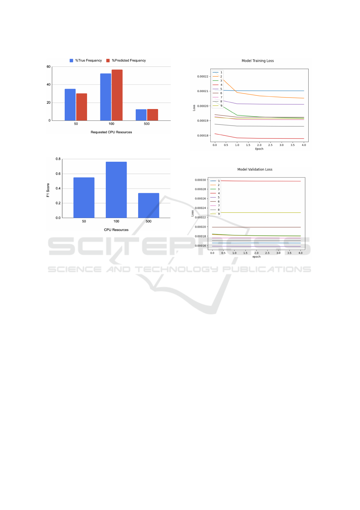
Figure 12: True and predicted frequency for grouped CPU

classes.

Figure 13: F1 score for grouped CPU classes.

5.2.2 Memory

When modeling memory resources for batch tasks,

we considered two options: 1) treating memory as

a standalone time series without any additional fea-

tures, and 2) incorporating CPU as a feature. To as-

sess the impact of CPU resources on improving the ef-

fectiveness of our predictive model, we calculated the

importance scores for the CPU feature. To do so, we

scaled the data using Min-Max between 0 and 1, ﬁt-

ted a linear regression model on the regression dataset

and extracted the coefﬁcients assigned to each input

variable (Artley, 2022). These coefﬁcients serve as

a basic measure of feature importance. The obtained

result of this analysis was 0.00392. As this value is

positive, it suggests that the inclusion of CPU values

does not hinder the learning process of our model. In-

stead, it indicates a minor positive inﬂuence of CPU

on predicting memory requirements. Consequently,

we decided to include CPU as a feature in our LSTM

model for memory prediction.

Our memory LSTM comprised of a single layer

with 32 hidden nodes and used the SGD optimizer

with a decaying learning rate of 0.001. The loss was

calculated using the Mean Squared Error (MSE) be-

tween the true and the predicted values. The loss for

different epochs and time series cross-validation splits

Figure 14: MSE training loss for memory.

Figure 15: MSE validation loss for memory.

for the training and validation sets can be observed in

Figure 14 and Figure 15, respectively.

The loss for the test data is 1.88e − 04 when the

values have been scaled between 0 and 1. Since the

original values of memory in the dataset are also nor-

malized and range between 0 and 100, we can simply

multiply the loss by 100 to get the loss for the original

data. The value is less than 1% in both the cases.

5.2.3 Lifetime

Task lifetimes are also predicted using an LSTM

model with regression. In order to assess the sig-

niﬁcance of resource requirements in determining the

duration of tasks, we once again calculated the im-

portance scores for CPU and memory features using

linear regression. Interestingly, we observed a nega-

tive score of −0.87 for CPU as a feature, indicating

its limited impact on predicting task lifetimes. On the

other hand, the memory feature exhibited a consider-

ably higher importance score of 350.26. One possible

explanation for this is the signiﬁcantly lower diversity

of unique values in the CPU data compared to mem-

ICPRAM 2024 - 13th International Conference on Pattern Recognition Applications and Methods

566

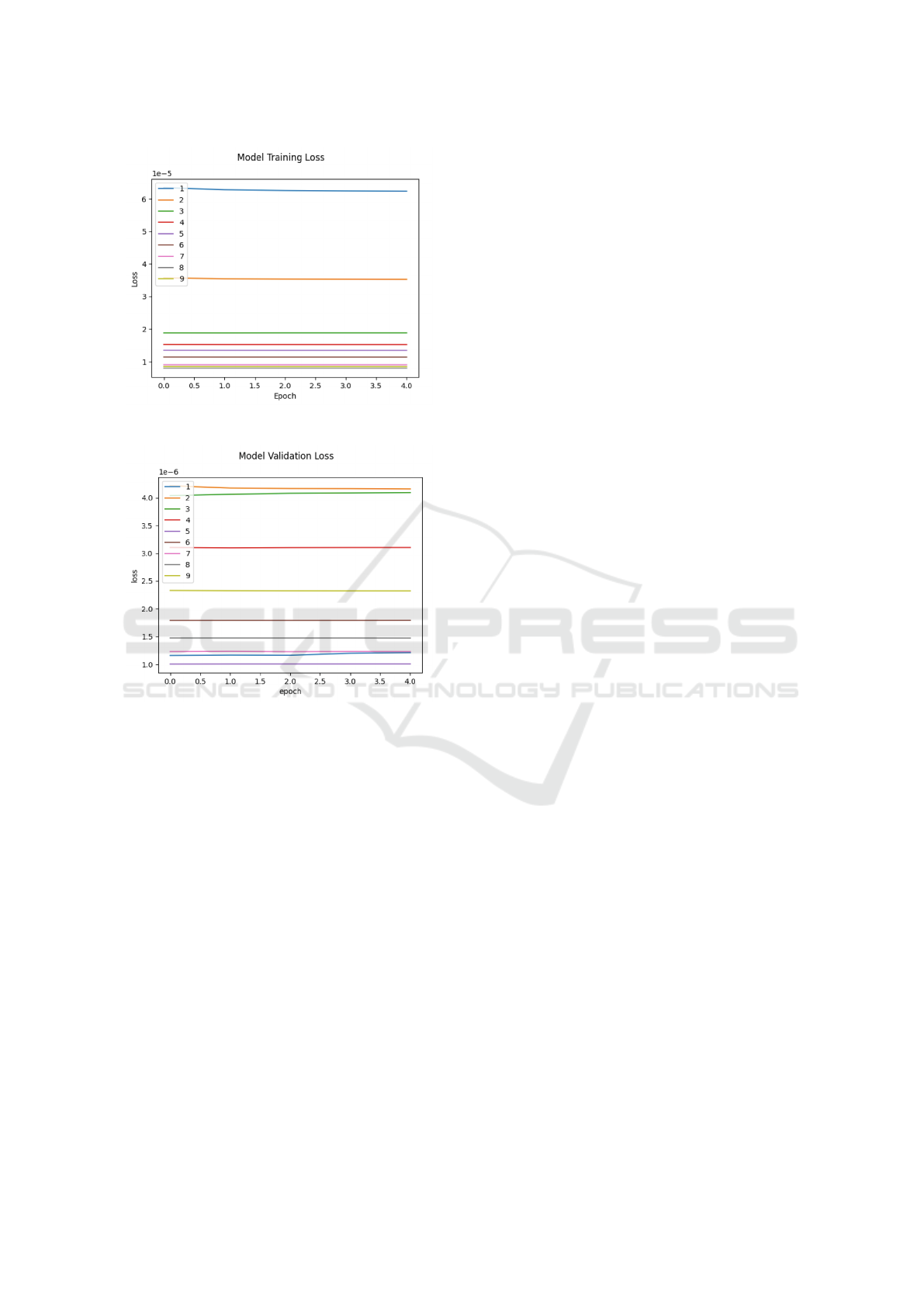
Figure 16: MSE training loss for lifetime.

Figure 17: MSE validation loss for lifetime.

ory. Within this limited set of CPU values, over 80%

of the data points have only two distinct values. These

two values may not be adequately useful for the life-

time model. Therefore, to model task lifetimes, we

included only the memory feature.

The LSTM model used for predicting task life-

times is similar to the one employed for modeling

memory. Both models utilize MSE losses during

training. The results for our training and validation

losses for the lifetime model are shown in Figure 16

and Figure 17, respectively. When evaluated on the

test data, which accounts for 25% of the dataset, our

model achieved a loss of 1.94e − 06. These results

demonstrate the high accuracy of our model in pre-

dicting task lifetimes.

6 CONCLUSION AND FUTURE

WORK

In this paper, we considered the problem of building a

predictive model for co-located tasks in a cloud com-

puting environment. We started by looking at the Al-

ibaba dataset that contains the following data for an

eight day period: (a) online and batch task arrivals

(co-located) (b) CPU and memory requirements for

each task (c) tasks lifetimes. We trained an ML model

using this dataset to predict the number of batch tasks

that arrive in a 30-minute window, the associated CPU

and memory requirements, and their lifetimes. We

used Seasonal ARIMA to predict the batch-task ar-

rival counts and three different LSTM networks to

predict CPU, memory and lifetime for an arriving

task. Our results show that our trained models ac-

curately forecast the number of batch task arrivals in

30-minute windows as well as their associated CPU,

memory requirements, and lifetimes.

In the future, we would like to generalize our pre-

diction model through the use of probabilistic gener-

ative models. A probabilistic model, e.g., to predict

the CPU resources, implies that we can sample from

a distribution over a valid set of CPU values. Hence,

our model will predict different sequences of CPU re-

quirements for different runs. Training a task sched-

uler using such a model will greatly enhance its ro-

bustness and generality.

REFERENCES

Alibaba (2018). Alibaba/clusterdata: Cluster data collected

from production clusters in alibaba for cluster man-

agement research.

Artley, B. (2022). Time Series Forecasting: Prediction In-

tervals. https://machinelearningmastery.com/cal

culate-feature-importance-with-python/. [Online;

accessed 23-February-2023].

Bahga, A., Madisetti, V. K., et al. (2011). Synthetic

workload generation for cloud computing applica-

tions. Journal of Software Engineering and Applica-

tions, 4(07):396.

Bergsma, S., Zeyl, T., Senderovich, A., and Beck, J. C.

(2021). Generating complex, realistic cloud work-

loads using recurrent neural networks. In Proceedings

of the ACM SIGOPS 28th Symposium on Operating

Systems Principles, SOSP ’21, page 376–391, New

York, NY, USA. Association for Computing Machin-

ery.

Brownlee, J. (2020). How to Calculate Feature Importance

With Python. https://towardsdatascience.com/time-s

eries-forecasting-prediction-intervals-360b1bf4b085.

[Online; accessed 5-March-2023].

Modeling Batch Tasks Using Recurrent Neural Networks in Co-Located Alibaba Workloads

567

Calheiros, R. N., Masoumi, E., Ranjan, R., and Buyya, R.

(2015). Workload prediction using arima model and

its impact on cloud applications’ qos. IEEE Transac-

tions on Cloud Computing, 3(4):449–458.

Calzarossa, M. C., Massari, L., and Tessera, D. (2016).

Workload characterization: A survey revisited. ACM

Comput. Surv., 48(3).

Chen, W., Ye, K., Wang, Y., Xu, G., and Xu, C.-Z. (2018).

How does the workload look like in production cloud?

analysis and clustering of workloads on alibaba cluster

trace. In 2018 IEEE 24th International Conference

on Parallel and Distributed Systems (ICPADS), pages

102–109.

Cheng, Y., Chai, Z., and Anwar, A. (2018). Characteriz-

ing co-located datacenter workloads: An alibaba case

study. In Proceedings of the 9th Asia-Paciﬁc Work-

shop on Systems, APSys ’18, New York, NY, USA.

Association for Computing Machinery.

Ching-Fu Chen, Y.-H. C. and Chang, Y.-W. (2009). Sea-

sonal arima forecasting of inbound air travel arrivals

to taiwan. Transportmetrica, 5(2):125–140.

Cortez, E., Bonde, A., Muzio, A., Russinovich, M., Fon-

toura, M., and Bianchini, R. (2017). Resource cen-

tral: Understanding and predicting workloads for im-

proved resource management in large cloud platforms.

In Proceedings of the 26th Symposium on Operating

Systems Principles, pages 153–167.

Da Costa, G., Grange, L., and de Courchelle, I. (2018).

Modeling, classifying and generating large-scale

google-like workload. Sustainable Computing: Infor-

matics and Systems, 19:305–314.

E. P. Box, G., M. Jenkins, G., C. Reinsel, G., and M. Ljung,

G. (1970). Time Series Analysis: Forecasting and

Control. Holden-Day, San Francisco.

Fattah, J., Ezzine, L., Aman, Z., Moussami, H. E., and

Lachhab, A. (2018). Forecasting of demand using

arima model. International Journal of Engineering

Business Management, 10:1847979018808673.

Grandl, R., Ananthanarayanan, G., Kandula, S., Rao, S.,

and Akella, A. (2014). Multi-resource packing for

cluster schedulers. In Proceedings of the 2014 ACM

Conference on SIGCOMM, SIGCOMM ’14, page

455–466, New York, NY, USA. Association for Com-

puting Machinery.

Guo, J., Chang, Z., Wang, S., Ding, H., Feng, Y., Mao, L.,

and Bao, Y. (2019). Who limits the resource efﬁciency

of my datacenter: An analysis of alibaba datacenter

traces. In 2019 IEEE/ACM 27th International Sympo-

sium on Quality of Service (IWQoS), pages 1–10.

Herbst, N. R., Huber, N., Kounev, S., and Amrehn, E.

(2013). Self-adaptive workload classiﬁcation and

forecasting for proactive resource provisioning. In

Proceedings of the 4th ACM/SPEC International Con-

ference on Performance Engineering, ICPE ’13, page

187–198, New York, NY, USA. Association for Com-

puting Machinery.

Hyndman, R. J. (2010). Forecasting with long seasonal pe-

riods. https://robjhyndman.com/hyndsight/longseas

onality/. [Online; accessed 15-January-2023].

Janardhanan, D. and Barrett, E. (2017). Cpu workload fore-

casting of machines in data centers using lstm recur-

rent neural networks and arima models. In 2017 12th

International Conference for Internet Technology and

Secured Transactions (ICITST), pages 55–60.

Jiang, C., Qiu, Y., Shi, W., Ge, Z., Wang, J., Chen, S., C

erin,

C., Ren, Z., Xu, G., and Lin, J. (2022). Characteriz-

ing co-located workloads in alibaba cloud datacenters.

IEEE Transactions on Cloud Computing, 10(4):2381–

2397.

Juan, D.-C., Li, L., Peng, H.-K., Marculescu, D., and

Faloutsos, C. (2014). Beyond poisson: Modeling

inter-arrival time of requests in a datacenter. In Tseng,

V. S., Ho, T. B., Zhou, Z.-H., Chen, A. L. P., and Kao,

H.-Y., editors, Advances in Knowledge Discovery and

Data Mining, pages 198–209, Cham. Springer Inter-

national Publishing.

Koltuk, F. and Schmidt, E. G. (2020). A novel method

for the synthetic generation of non-i.i.d workloads for

cloud data centers. In 2020 IEEE Symposium on Com-

puters and Communications (ISCC), pages 1–6.

Liu, Q. and Yu, Z. (2018). The elasticity and plasticity

in semi-containerized co-locating cloud workload: A

view from alibaba trace. In Proceedings of the ACM

Symposium on Cloud Computing, SoCC ’18, page

347–360, New York, NY, USA. Association for Com-

puting Machinery.

Mishra, S. (2020). Methods for Normality Test with Appli-

cation in Python. https://towardsdatascience.com/m

ethods-for-normality-test-with-application-in-pyt

hon-bb91b49ed0f5. [Online; accessed 15-February-

2023].

Mitrani, A. (2020). Time Series Decomposition and

Statsmodels Parameters. https://towardsdatascien

ce.com/time-series-decomposition-and-statsmodels

-parameters-69e54d035453. [Online; accessed 19-

January-2023].

Moreno, I. S., Garraghan, P., Townend, P., and Xu, J.

(2014). Analysis, modeling and simulation of work-

load patterns in a large-scale utility cloud. IEEE

Transactions on Cloud Computing, 2(2):208–221.

Reiss, C., Wilkes, J., and Hellerstein, J. L. (2011). Google

cluster-usage traces: format+ schema. Google Inc.,

White Paper, 1:1–14.

Siami-Namini, S., Tavakoli, N., and Siami Namin, A.

(2018). A comparison of arima and lstm in fore-

casting time series. In 2018 17th IEEE International

Conference on Machine Learning and Applications

(ICMLA), pages 1394–1401.

Tirmazi, M., Barker, A., Deng, N., Haque, M. E., Qin,

Z. G., Hand, S., Harchol-Balter, M., and Wilkes, J.

(2020). Borg: the next generation. In Proceedings

of the ﬁfteenth European conference on computer sys-

tems, pages 1–14.

Verma, A., Korupolu, M., and Wilkes, J. (2014). Evaluating

job packing in warehouse-scale computing. In 2014

IEEE International Conference On Cluster Comput-

ing (CLUSTER), pages 48–56, Los Alamitos, CA,

USA. IEEE Computer Society.

Xu, R., Mitra, S., Rahman, J., Bai, P., Zhou, B., Bronevet-

sky, G., and Bagchi, S. (2018). Pythia: Improving

ICPRAM 2024 - 13th International Conference on Pattern Recognition Applications and Methods

568

datacenter utilization via precise contention prediction

for multiple co-located workloads. In Proceedings of

the 19th International Middleware Conference, Mid-

dleware ’18, page 146–160, New York, NY, USA. As-

sociation for Computing Machinery.

Yu Wang, Chunheng Wang, C. S. and Xiao, B. (2018).

Short-term cloud coverage prediction using the arima

time series model. Remote Sensing Letters, 9(3):274–

283.

Zhang, Y., Yu, Y., Wang, W., Chen, Q., Wu, J., Zhang, Z.,

Zhong, J., Ding, T., Weng, Q., Yang, L., Wang, C., He,

J., Yang, G., and Zhang, L. (2022). Workload consol-

idation in alibaba clusters: The good, the bad, and the

ugly. In Proceedings of the 13th Symposium on Cloud

Computing, SoCC ’22, page 210–225, New York, NY,

USA. Association for Computing Machinery.

Modeling Batch Tasks Using Recurrent Neural Networks in Co-Located Alibaba Workloads

569