OCT Image Analysis of Internal Changes in Leaves due to Ozone

Stresses

Hayate Goto

, Nofel Lagrosas

and Tatsuo Shiina

Chiba University, Yayoi-cho, Inage-ku, Chiba-shi, Chiba, Japan

School of Engineering, Kyushu University, 744 Motooka, Nishi-ku, Fukuoka, Japan

Keywords: OCT, Indicator Plant, Environmental Assessment, Ozone, GLCM.

Abstract: Changes in environmental conditions can be evaluated by detecting the conditions in indicator plants.

Indicator plants are sensitive to specific environmental stresses. This research focused on white clover as an

indicator plant for ozone. To analyze the effects of weaker stresses, compact OCT (Optical coherence

tomography) for plants was developed, which allows for non-invasive and non-contact cross-sectional

imaging of white clover (Trifolium repens) leaves exposed to ozone gas. OCT image changes on each level

of ozone damage were evaluated using parameters such as the OCT signal level of the leaf palisade layer, the

thickness of the leaf palisade layer, and texture analysis using GLCM (Gray-Level Co-occurrence Matrix).

Measurements of leaves grown in our laboratory showed increased palisade tissue signal, thicker palisade

tissue, a smaller distribution of palisade layer thickness, increased OCT image contrast, and decreased OCT

image homogeneity.

1 INTRODUCTION

In Japan, due to the pollution problems caused by

high economic growth around the 1950s, it became

clear that plants were affected by air pollution

(Takeshi, 2020). Using plants to help evaluate the

atmospheric environment is attracting attention.

Indicator plants are sensitive to specific

environmental stresses which can provide vital

information on the local environmental conditions.

For example, white clover is an indicator plant for

ozone, and white spots of visible damage occur near

the leaf’s main veins when exposed to high

concentrations of ozone gas. Ozone concentrations

can be high in urban areas due to the influence of

traffic. There are significant differences in ozone

concentrations between rural and urban areas.

The white clover in the field is greatly affected by

ozone, and it is possible to quickly estimate the

environment by observing its leaves. Indicator plants

are generally evaluated by visual inspection, satellite

observation, and spectroscopic observation.

Spectroscopic observations can observe a decrease in

https://orcid.org/0000-0001-5387-9109

https://orcid.org/0000-0002-8672-4717

https://orcid.org/0000-0001-9292-4523

the chlorophyll of the plants. However, this

phenomenon is caused by dryness, insect damage,

and nutritional deficiencies, and it is challenging to

elucidate the cause of the change in the experimental

results(Takeshi, 2020).

Optical coherence tomography (OCT) can detect

morphological and intracellular tomographic images

using near-infrared light (Huang et al., 1991). The

internal change in plants is related to specific

environmental stresses or diseases. Additionally,

since OCT is an in-situ and non-invasive technique, it

can be used to observe indicator plants in long-term

changes over time (Wijesinghe et al., 2017; Lee et al.,

2019). Recent studies showed that OCT is used in

ophthalmology (Drexler et al., 2001; Wojtkowski et

al., 2005; Chopra, 2022), dentistry (Sinescu et al.,

2008; Colston et al., 1998), and dermatology (Liu et

al., 2020; Gambichler et al., 2005). OCT is also used

for observation of seed germination process (De Silva

et al., 2021; Saleah et al., 2022) and diagnosis of

vegetables and fruits (Zhou et al., 2022; Saleah et al.,

2022; Gocławski et al., 2017). Compared to

technologies that visualize internal structures, such as

Goto, H., Lagrosas, N. and Shiina, T.

OCT Image Analysis of Internal Changes in Leaves due to Ozone Stresses.

DOI: 10.5220/0012392200003651

Paper published under CC license (CC BY-NC-ND 4.0)

In Proceedings of the 12th International Conference on Photonics, Optics and Laser Technology (PHOTOPTICS 2024), pages 65-71

ISBN: 978-989-758-686-6; ISSN: 2184-4364

MRI and X-rays, OCT is high resolution, and capa

ble of non-invasive quantitative analysis. Since the

developed OCT is compact to bring outside, plant

internal structures can be measured at growing area.

Environmental conditions can assess to measuring the

indicator plant in the growth area.

Ozone is purposely absorbed by the plant through

its stomata which destroys the palisade tissue near the

adaxial epidermis. In our previous study, white clover

was exposed to high concentrations of ozone gas, and

it was confirmed that the OCT signal decreased

measured above the palisade tissue (Goto et al., 2023).

To evaluate the internal changes caused by ozone, this

research extracted features from the OCT images of

white clover leaves.

This study aimed to explore OCT signal

processing and image analysis methods for

classifying the level of environmental damage to

white clover leaves using machine learning. Since the

effect of ozone gas is likely to appear in the thickness

and OCT image texture of the palisade tissue, we

performed thickness evaluation by layer detection

using peak detection and OCT image texture analysis

and developed the optimum feature extraction for

OCT signal analysis.

2 METHOD

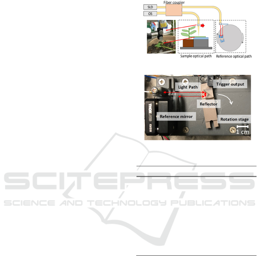
2.1 Developed Plant OCT System

The developed plant time domain (TD)-OCT system

is based on a Michelson interferometer (Fig.1). The

light irradiated from the super luminescent diode

(SLD (ANRITSU, AS3E113HJ10M)) light source is

split into a reference optical path and a sample optical

path by a fiber coupler. The light returning from the

sample optical path has different optical path lengths

due to the light backscattered by different layers

within the sample leaf. The reference optical path

length changes at a constant speed, performing the

rotation mechanism (Fig.2). The light path in the

reference optical path (red arrow) is shown in Figure

2. The light comes from the light upper position,

returns to the same position, and goes back to the fiber

coupler. To rotate the mirror on the stage, the

reference optical path length is changed. Since low-

coherence light is used, the intensity of the

interference light can be observed only when the

optical path lengths match within the coherence

length. Since the reference optical path length

changes linearly with time, linear analysis can be

conducted directly (Shiina et al., 2003; Saeki et al.,

2021).

Figure 1: The configuration of the plant OCT system.

Figure 2: Reference optical path system.

Table 1: Specification of OCT system.

Parameters Values

Center wavelength 1310 nm

FWHM 53 nm

SLD output 15μW

Axial resolution 14.2 μm

Lateral resolution 10 μm

A-scan rate 25 Hz

OCT size 198×168×98 mm

Probe size φ6 mm×9 mm

Table 1 shows the characteristics of the developed

OCT (Goto et al., 2023). The central wavelength is

1310 nm, which has low absorption by chlorophyll

and the local minimum value of the absorption by

water. The axial resolution is 14.2 μm related to SLD

coherent length. At 1310 nm, the resolution is lower

than that of light wavelength around 800 nm, which

is commonly used in medical OCT, but the measuring

depth is more extended because it is less affected by

scattering and absorption. The signal acquisition rate

is 25 Hz, and 16 accumulated signals were averaged

to collect one A-line data which reduces noise. The

probe moves every 10 μm to produce an image from

400 signals. The size of OCT is small enough to be

carried outside and measured in the field.

PHOTOPTICS 2024 - 12th International Conference on Photonics, Optics and Laser Technology

2.2 Exposure to Ozone Gas

White clover was grown in an incubator at 20℃ with

an ozone generator (KENWOOD, CAX-DM01) at a

concentration of 0.17-0.21 ppm. The red and blue

light of the cold cathode lamp that is easy to absorb

by plant’s leaves is irradiated for 15 hours a day inside

the incubator. Measurements were done before

placing plants in the incubator and after placing plants

in the incubator every 3, 6, 10, and 14 days. The

plants were measured in growing conditions to

analyze effects within the same leaf.

2.3 Parameter Extraction

To confirm the influence of ozone, multiple analysis

parameters were utilized by measuring the intensity

of the OCT signal, the thickness of the palisade

structure using peak detection, and texture analysis

using the Gray-Level Co-occurrence Matrix (GLCM)

within the palisade structure.

2.3.1 The Intensity of Palisade Tissue

To obtain the OCT interference intensity of the

palisade tissue, the acquired data was processed by

background subtraction, focal length correction, and

distance squared correction. To make one A-line, 400

A-lines were aligned and averaged. The averaged A-

line was performed by using normalization with the

maximum value, and logarithmic transformation.

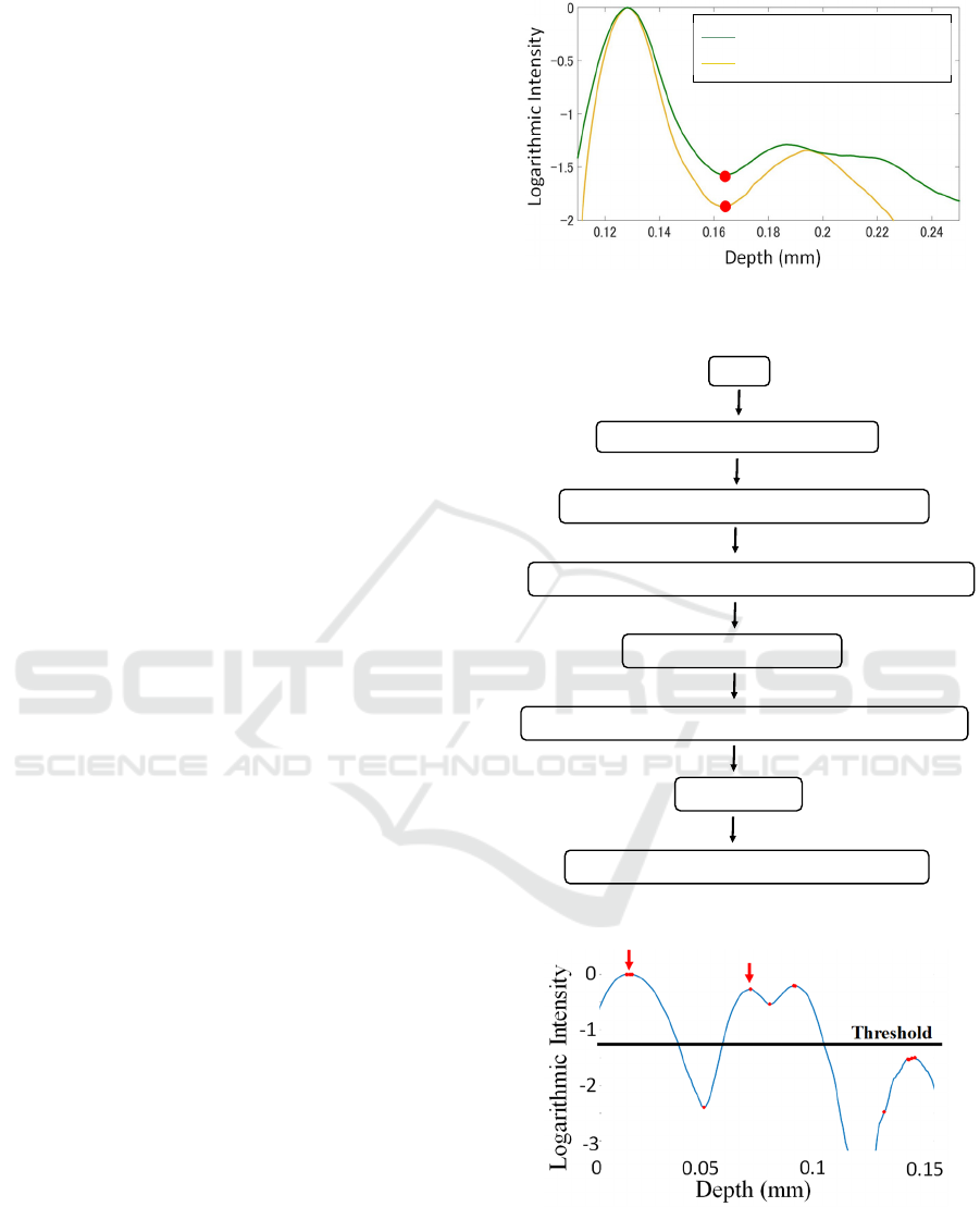
Figure 3 shows the OCT signal change in the A-line

before and after 10 days of exposure to ozone gas.

The x-axis is the depth of the sample leaves, and the

y-axis is the logarithmic intensity of the OCT signal.

The green line in Fig.3 is before exposure to ozone,

the yellow line is after ten days of exposure to ozone.

This graph shows smooth lines because averaging to

evaluate the change in a whole image of a leaf itself.

The first minimum value after the maximum position

(red dots points in Fig. 3) was defined as the intensity

of the middle position of the palisade layer.

2.3.2 Thickness Calculations

Figure 4 shows the flowchart of the thickness

calculation program. This program selects the

positions of the first and second peaks. Since the first

peak is the surface layer, and the second peak is the

palisade and spongy layer boundary, the difference

between these peaks is considered as the palisade

layer thickness.

Peak detection was performed using Matlab’s

PeakFinder command (Fig.5). The x-axis shows the

depth information of the leaf, and the y-axis shows

Figure 3: The signal comparison in the palisade layer before

and after exposed to ozone gas.

Figure 4: Flowchart of thickness calculations.

Figure 5: Peak detection of A-line.

the logarithmic intensity of the OCT signal. At this

time, a threshold value was used to prevent peaks

below a particular value. After that, all of the A-line

peaks in the OCT images were detected. The outliers

START

Find the peaks positon and intensity

Group peaks with peak location difference < 100

Select the maximum of signals at first group as the 1

peak

Select next peak as 2

peak

Interpolate the average of the adjacement value to outliers

Moving average

Calculate the distance between 1

and 2

peak

Before exposure to ozone

After 10 days exposure to ozone

OCT Image Analysis of Internal Changes in Leaves due to Ozone Stresses

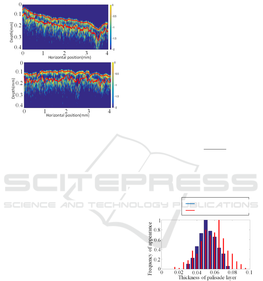
Figure 6: Peak detection of B-scan image (a) Before

exposure to ozone gas and (b) After 10 days exposure to

ozone gas.

of peak positions in the images were removed and

interpolated. The moving average was taken so the

peak detection results fit smoothly with the

OCTimage. Finally, we obtained the distance

between the two peaks and made a histogram. The red

arrow indicates the peak point that is defined by this

method.

Figure 6(a) and 6(b) show the results of peak

detection before and after exposure to ozone gas,

respectively. The image's upper part is the leaf's

adaxial surface, and measurements are taken with

light incident from this direction. The x-axis is the

scanning direction, and the y-axis is the depth

direction of the white clover leaf. The image's aspect

ratio has been changed to make it easier to see peak

detection results. The red line in the image is the

result of peak detection, and it can be confirmed that

the two layers can be detected correctly. Since the

ozone gas destroys the palisade tissue, the two peaks

in Figure 6(b) have a larger distance than the two

peaks in Figure 6(a).

From each histogram, the kurtosis, which

indicates the degree of concentration of the

distribution, and the average value were obtained and

compared with the measurement results of white

clover leaves grown under each condition.

Figure 7 is an example of the histogram. The blue

bar graph is the result before exposure to ozone gas,

and the red bar graph is the result after 10 days of

exposure to ozone gas. A detailed discussion of

Figure 7 is shown in subsection 3.2 Thickness

calculation.

2.3.3 GLCM (Gray-Level Co-Occurrence

Matrix)

GLCM is a method that creates a matrix from the

frequency of appearance of specific pixel value pairs

and evaluates the image texture of an object. In the

previous OCT research, OCT images could evaluate

the moisture change because of the storage using

contrast, correlation, energy, and homogeneity from

the GLCM matrix and classify them using machine

learning of support vector machine (SVM)

(Srivastava et al., 2018).

Figure 8 shows the method for making GLCM.

One pixel intensity compares with the intensities of

adjacent pixels. GLCM creates a matrix that counts

the number of identical intensity pairs. Contrast and

homogeneity were calculated using the following

equations (1) and (2) using the created matrix.

Contrast  

𝑖𝑗



𝑝



𝑖,𝑗



,

(1)

Homogeneity 

𝑝𝑖,𝑗

1|𝑖𝑗|

(2)

The i,j indicates the positions within the GLCM

matrix, and p(i,j) indicates the frequency of

appearance of specific pixel value pairs. μ and σ are

each row and column's average and standard

deviation, respectively.

Figure 7: Histgram of the thickness.

3 RESULTS AND DISCUSSION

3.1 Intensity of Palisade Layer

Figure 9 shows the result of the intensity change

inside the palisade tissues. The vertical axis indicates

the differences between the epidermis surface and the

middle position of palisade tissue intensity, and the

horizontal axis is the day of growing in the incubator.

Before exposure to ozone

After 10 days exposure to ozone

(a)

(b)

PHOTOPTICS 2024 - 12th International Conference on Photonics, Optics and Laser Technology

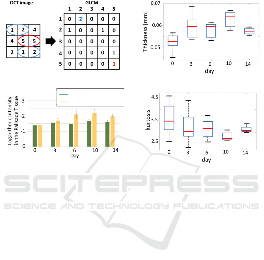
Figure 8: GLCM.

Figure 9: Average of thickness.

The yellow bar indicates the result of growth in

the high concentration of ozone gas, and the green bar

indicates the result of growth in the normal air

condition. Higher intensities are observed in the

palisade tissues under high ozone concentration as

compared to tissues under normal air conditions.

In the case of normal conditions, the intensity of

palisade tissue did not have significant changes.

However, in the case of a high ozone concentration,

the palisade tissue intensity became higher from Day

0 to Day 10. Ozone gas enters the inside of leaves

from the stoma and generates the reactive oxygen

species (Takeshi, 2020). Since the oxidation stress

occurs due to the reactive oxygen species, the

palisade tissue is highly affected by ozone as

compared to spongy tissue. The less scattering effect

observed inside the destroyed leaf palisade tissue

leads to a lower signal.

Comparing the ozone exposure result of Day 0

with other days except for Day 10 in Figure 9 using a

t-test, a significant change didn’t appear in the normal

air conditions (Day 3 : p = 0.140, Day 6 : p = 0.460,

Day 10 : p = 0.021, Day 14 : p = 0.059). Day 10 result

shows a significant change compared to Day 0

because of the growth or senescence. On the other

hand, a significant change was observed from Day 0

to later days (Day 3: p = 0.037, Day 6 : p = 0.047, Day

10 : p = 0.012, Day 14 : p = 0.000064) after exposure

Figure 10:

Average thickness.

Figure 11: Kurtosis of thickness distribution.

to ozone gas. In this research, visible inspection

where white spots appear near the leaf's main vein can

be observed after 10 days of exposure to ozone gas.

Thus, the indicator plants measurement using OCT

can detect the leaf change after 3 days of exposure to

ozone gas, and it is earlier than visible inspection.

OCT can detect the early stage of the inspection and

small inspection due to environmental stresses or

diseases.

3.2 Thickness Calculations

Figure 7 shows the histogram of leaf thickness after 0

and 10 days of exposure to ozone gas. This thickness

value was calculated as described in subsection ‘2.3.2

Thickness calculations’ in the section ‘2 METHOD’.

The median value of the thickness in 10 days became

thicker than the median value in 0 days. The 10-day

histogram has a wider distribution than the 0-day

histogram due to the ozone gas effect.

Figures 10 and 11 show the average and kurtosis

of the thickness measured from the OCT image,

respectively. The horizontal axis is the day of

growing in the incubator, and the vertical axis is the

average and kurtosis of the thickness. As observed,

the average thickness increases, and the kurtosis

decreases during the sampling period. Since the part

of destroyed tissue by ozone was filled with water, the

Growing at normal atmosphere

Growing at ozone atmosphere

OCT Image Analysis of Internal Changes in Leaves due to Ozone Stresses

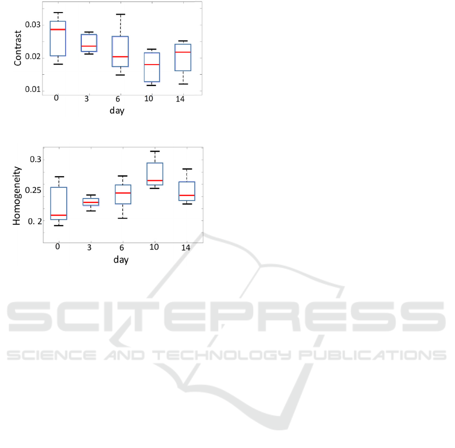
Figure 12: Contrast of palisade layer.

Figure 13: Homogeneity of palisade layer.

intercellular space expanded, and the thickness of

palisade tissue increased as shown in Figure 10. The

decrease of kurtosis is due to the morphological

changes in the leaf. As the influence of the ozone

effect increased, the damaged region in the leaf

expanded and made a uniform condition. This caused

a decrease in the distribution of thickness, and the

kurtosis was decreased. The leaf at the initial state has

a large variation of the kurtosis. The initial state of

cells that are not damaged and have several

conditions due to senescence. Additionally, the 14th-

day result of an average thickness is increased, and

the kurtosis of thickness distribution is decreased. It

did not fit the same trend in earlier days.

3.3 GLCM

Figures 12 and 13 show the GLCM results of contrast

and homogeneity, respectively. The horizontal axis is

the day of growing in the incubator, and the vertical

axis is the contrast and homogeneity. The contrast

value is decreased and the homogeneity value is

increased with the day except for 14 days result.

These results showed a similar trend to the thickness

results (Fig. 10 and 11). This confirms that the

palisade tissues were destroyed and filled with water

upon exposure to ozone gas. As observed in the OCT

images, the water part showed less contrast and high

homogeneity compared with the cell part.

Day 14 has the other trend same as Figures 10 and

11 such as high contrast and less homogeneity. The

plants may become partially senescence by the ozone

effect. Since this causes the dryness inside the leaf

and the high scattering of the light, the thickness

became thicker (Fig.10), bigger kurtosis of thickness

(Fig.11), high contrast (Fig.12), and low homogeneity

(Fig.13).

4 CONCLUSIONS

In this study, we examined the possibility of the white

clover leaves as an indicator plant for ozone gas using

TD-OCT. This study shows the use of OCT as an

early detection device for ozone gas. If the plant

leaves are exposed to ozone gas, ozone gas enters

inside the leaves from the stoma and destroys the

palisade tissue. This phenomenon causes the OCT

intensity to decrease in the palisade tissue. This study

performed peak detection and texture analysis to

evaluate the effects of ozone gas on white clover

leaves. Additionally, the thickness of palisade tissue

became thicker and has smaller distribution. The

GLCM result of palisade tissue has low contrast and

high homogeneity. After 14 days of exposure to

ozone gas, due to necrosis, they showed other trends

compared to before 14 days.

To classify the degree of damage caused by ozone

gas, this research will increase the number of samples

and use machine learning for classification. To

distinguish the ozone effect from other stresses, the

plants will be measured and evaluated under other

conditions such as dryness, lack of nutrients, lack of

light, and varying temperatures. The parameters such

as interfered intensity of palisade tissue, thickness

distribution of the palisade tissue, and image texture

that only appeared in the ozone effect will be selected

for evaluation of the condition of the plant growing

area.

Using OCT in the field, the relationship between

the field conditions and indicator plant parameters

can be properly assessed. This method can be helpful

in the field of agriculture research because the

selection of crops to be planted, and proper

application of pesticides and other growth parameters

can be studied.

ACKNOWLEDGMENTS

This work was supported by JST, the establishment

of university fellowships towards the creation of

PHOTOPTICS 2024 - 12th International Conference on Photonics, Optics and Laser Technology

science and technology innovation, Grant Number

JPMJFS2107.

REFERENCES

Takeshi, I. (2020). Atmospheric environment and Plant

(Taiki kankyo to syokubutu. Asakura Shoten, ISBN

987-4-254-42045-6 C 3061 ,Japan.

Huang, D., Swanson, E. A., Lin, C. P., Schuman, J. S.,

Stinson, W. G., Chang, W., Hee, M. R., Flotte, T.,

Gregory, K., & Puliafito, C. A. (1991). Optical

coherence tomography. Science (New York, N.Y.),

254(5035), 1178–1181.

Drexler, W., Morgner, U., Ghanta, R. K., Kärtner, F. X.,

Schuman, J. S., & Fujimoto, J. G. (2001). Ultrahigh-

resolution ophthalmic optical coherence tomography.

Nature medicine, 7(4), 502–507.

Wojtkowski, M., Srinivasan, V., Fujimoto, J. G., Ko, T.,

Schuman, J. S., Kowalczyk, A., & Duker, J. S. (2005).

Three-dimensional retinal imaging with high-speed

ultrahigh-resolution optical coherence tomography.

Ophthalmology, 112(10), 1734–1746.

Chopra V. (2022). Association of Rates of Optical

Coherence Tomography Angiography Vessel Density

Loss on Initial Visits With Future Visual Field

Progression. JAMA ophthalmology, 140(4), 326–327.

Sinescu, C., Negrutiu, M. L., Todea, C., Balabuc, C., Filip,

L., Rominu, R., Bradu, A., Hughes, M., & Podoleanu,

A. G. (2008). Quality assessment of dental treatments

using en-face optical coherence tomography. Journal of

biomedical optics, 13(5), 054065.

Colston, B., Sathyam, U., Dasilva, L., Everett, M., Stroeve,

P., & Otis, L. (1998). Dental OCT. Optics express, 3(6),

230–238.

Liu, Y., Zhu, D., Xu, J., Wang, Y., Feng, W., Chen, D., Li,

Y., Liu, H., Guo, X., Qiu, H., & Gu, Y. (2020).

Penetration-enhanced optical coherence tomography

angiography with optical clearing agent for clinical

evaluation of human skin. Photodiagnosis and

photodynamic therapy, 30, 101734.

Gambichler, T., Moussa, G., Sand, M., Sand, D., Altmeyer,

P., & Hoffmann, K. (2005). Applications of optical

coherence tomography in dermatology. Journal of

dermatological science, 40(2), 85–94.

De Silva, Y. S. K., Rajagopalan, U. M., Kadono, H., & Li,

D. (2021). Positive and negative phenotyping of

increasing Zn concentrations by Biospeckle Optical

Coherence Tomography in speedy monitoring on lentil

(Lens culinaris) seed germination and seedling growth.

Plant Stress, 2, 100041.

Saleah, S. A., Lee, S. Y., Wijesinghe, R. E., Lee, J., Seong,

D., Ravichandran, N. K., Jung, H. Y., Jeon, M., & Kim,

J. (2022). Optical signal intensity incorporated rice seed

cultivar classification using optical coherence

tomography. Computers and Electronics in Agriculture,

198, 107014.

Zhou, Y., Wu, Y., & Chen, Z. (2022). Detection of Mold-

Contaminated Maize Kernels Based on Optical

Coherence Tomography. Food Anal. Methods, 15,

1619-1625.

Saleah, S. A., Wijesinghe, R. E., Lee, S. Y., Ravichandran,

N. K., Seong, D., Jung, H. Y., Jeon, M., & Kim, J.

(2022). On-field optical imaging data for the pre-

identification and estimation of leaf deformities.

Scientific data, 9(1), 698.

Gocławski, J., Nalewajko, J. S., Korzeniewsk, E.,&

Piekarsk, A. (2017). The use of optical coherence

tomography for the evaluation of textural changes of

grapes exposed to pulsed electric field. Computers and

Electronics in Agriculture, 142, 29-40.

Wijesinghe, R. E., Lee, S. Y., Ravichandran, N. K., Han, S.,

Jeong, H., Han, Y., Jung, H. Y., Kim, P., Jeon, M., &

Kim, J. (2017). Optical coherence tomography-

integrated, wearable (backpack-type), compact

diagnostic imaging modality for in situ leaf quality

assessment. Applied optics, 56(9), D108–D114.

Lee, J., Lee, S. Y., Wijesinghe, R. E., Ravichandran, N. K.,

Han, S., Kim, P., Jeon, M., Jung, H. Y., & Kim, J.

(2019). On-Field In situ Inspection for Marssonina

Coronaria Infected Apple Blotch Based on Non-

Invasive Bio-Photonic Imaging Module. IEEE Access,

7, 148684-148691.

Goto, H., & Shiina, T. (2023). Environmental Pollution

Assessment with Indicator Plant Under Ozone Gas

Atmosphere by Using OCT. Proceedings of the 11th

International Conference on Photonics, Optics and

Laser Technology, 1, PHOTOPTICS, 34-39.

Shiina, T., Moritani, Y., Ito, M., & Okamura, Y. (2003).

Long-optical-path scanning mechanism for optical

coherence tomography. Applied optics, 42(19), 3795–

3799.

Saeki, K., Huyan, D., Sawada, M., Nakamura, A., Kubota,

S., Uno, K., Ohnuma, K., & Shiina, T. (2021). Three-

dimensional measurement for spherical and

nonspherical shapes of contact lenses. Applied optics,

60(13), 3689–3698.

Srivastava, V., Dalal, D., Kumar, A., Prakash, S., & Dalal,

K. (2018). In vivo automated quantification of quality

of apples during storage using optical coherence

tomography images. Laser Physics, 28, 066207

OCT Image Analysis of Internal Changes in Leaves due to Ozone Stresses