An Alternative Robust Design to Assist a Single-Objective
Performance Optimization: Simulation Analysis of a Flexible
Manufacturing System
Wa-Muzemba Anselm Tshibangu
Department of Industrial and Systems Engineering, Morgan State University, 1700 E. Cold Spring Lane, Baltimore,
Maryland 21251, U.S.A.
Keywords: Flexible Manufacturing System (FMS), Discrete-Event Simulation, Taguchi, Design of Experiments (DOE),
Robust Design, Single-Objective Optimization, ANOVA, T-Test, Normal Probability Plot.
Abstract: During the lockdowns following the Covid-19 pandemic many companies have become flexible by
implementing new manufacturing technologies, such as group technology (GT), just-in-time (JIT) production
systems, and flexible manufacturing systems (FMSs) that, hence, become among the solutions of the future.
This paper uses the emergence of these systems to present an alternative robust design formulation to Taguchi
methodology before proposing a single-objective optimization scheme to find the optimal operational settings
of primary individual key performance indicators (KPIs). The study uses the Throughput Rate (TR) and the
Mean Flow Time (MFT) as illustrative examples of KPIs, tracked over a range of AGV fleet sizes. Additional
KPIs, e.g., Work-in-process (WIP), Machine utilization, and AGV utilization are also analyzed as secondary
measures to validate and fine-tune the results of the procedure. The study deploys and uses in association
multiple statistical tools for a proper analysis and validation of the technique. The effectiveness of the
proposed model is validated by comparing the results to some other similar approaches. Although derived
from simulation of manufacturing operations, the framework presented in this paper can be applied to various
industries including food production, financial institutions, warehouse industry, and healthcare.
1 INTRODUCTION
The COVID-19 pandemic put forth the role of
technology in everyday business, especially in the
manufacturing operations. Products needed to be
manufactured quicker without sacrificing quality
standards. The situation raised the demand for rare
production items such as ventilators, gloves, face
shields, masks, paper towels, toilet papers,
a n d sanitizers at a high rate (Cohen, 2020).
M anufacturing giants such as General Motors and
Ford Motor Company turned their production
systems to support the need of society in terms of
manufacturing ventilators (Aalok Kumar et al., 2020).
Then, it became evident that a flexible manufacturing
system (FMS) was inevitable to fulfil the requirement
for such necessary items. Today, in the post pandemic
era, national government institutions, health
institutions, food processing industry, pharmaceutical
manufacturing organizations, should be prepared in
advance to tackle any situation to control the
production of essential and nonessential items during
a pandemic, and have sufficient buffer plans to
address the availability of life saver stocks such as
ventilators, vaccines, sanitizers, masks, and face
shields (Aalok Kumar et al., 2020) and also, a variety
of non-health related goods, e.g., food, tools,
automobile parts, and other equipment.
The choice of performance measures in a
processing system such an FMS depends highly on
management policy and decision-making approach,
especially under COVID-19-lke supply chain
disruption conditions. Multiple objective measures,
often referred to as Key Performance Indicators
(KPIs) are needed to describe the dynamic nature of
a manufacturing or production system such as an
FMS.
A single performance measure is not enough to
capture and characterize the overall performance of a
system. Hence, optimizing a system with respect to
one single objective only may lead to sacrificing other
objective(s) of interest. For example, the objective of
Tshibangu, W.
An Alternative Robust Design to Assist a Single-Objective Performance Optimization: Simulation Analysis of a Flexible Manufacturing System.
DOI: 10.5220/0012392100003639
Paper published under CC license (CC BY-NC-ND 4.0)
In Proceedings of the 13th International Conference on Operations Research and Enterprise Systems (ICORES 2024), pages 309-316
ISBN: 978-989-758-681-1; ISSN: 2184-4372
Proceedings Copyright © 2024 by SCITEPRESS – Science and Technology Publications, Lda.
309

minimizing in-process inventory might conflict with
that of maximizing a production rate.
However, the author believes that during
conditions of supply chain disruptions like the past
pandemic era, it may become strategical to prioritize
only one single performance to the detriment of
others depending on the industry segment. Therefore,
this paper presents a unique robust design scheme
applied to an FMS with the objective of proposing a
single-objective performance optimization procedure
as well as all the statistical validation tools that
support the scheme.
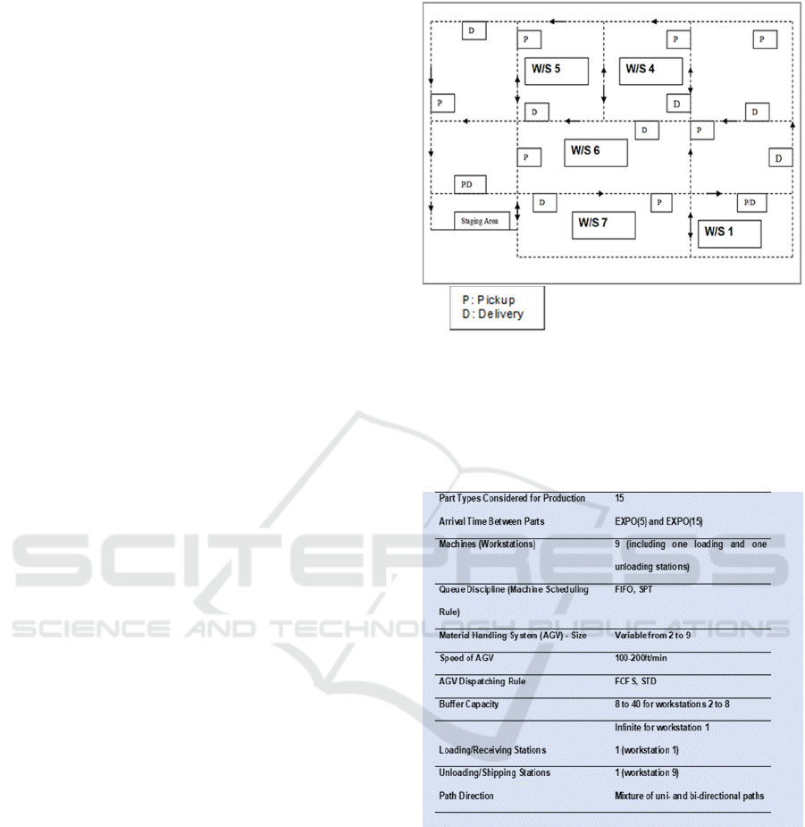
2 THE HYPOTHETICAL FMS
The paper analyzes a hypothetical flexible
manufacturing system (FMS) using discrete-event
simulation. The study proposes a unique and robust
scheme in designing, modeling, and optimizing the
system. The system is modeled with a total number of
9 workstations including a receiving and a shipping
station. This 9-station flexible manufacturing system
as schematically depicted in Figure 1 is served by a
fleet of AGVs while processing fifteen-part types,
each with a different processing time.
The study analyzes and proposes a single criteria
“empirical” optimization scheme that is subsequently
and separately applied to two most popular and
conflicting performance measures indicators, namely,
the Throughput Rate (TR) and the Mean Flow Time
(MFT), over a range of AGV fleet sizes. The
proposed optimization procedure also deploys a
series of additional statistical tools intended to
support the validation of the approach. Besides, three
other metrics are tracked and analyzed as secondary
measures or benchmarks to validate the selection of
optimal values. The proposed optimization scheme is
developed by studying an AGV-served FMS and
evaluating its overall performance while considering
5 design parameters as controllable variables,
designated by X
i
(i=1…5), namely:
i) the number of AGVs (X
1
),
ii) the speed of AGV (X
2
),
iii) the queue discipline (X
3
), iv) the AGV
dispatching rule (X
4
), v) and the buffer size
(X
5
). These variables have a direct impact on
the performance of machines and material
handling (AGVs), considered as the most
expensive components of the overall system.
Figure 1: The Hypothetical Flexible Manufacturing
System.
Table 1 depicts the shop configuration as studied
in this paper.
Table 1: FMS – Shop Configuration.
3 OVERVIEW
The COVID-19 pandemic has disrupted
manufacturing and production operations around the
world on a huge scale, challenging manufacturers,
vendors, and suppliers to seek for innovative new
ways to continue their operations safely while
minimizing risks and disruptions (Cappelli et al.,
2020).
Manufacturing becomes increasingly digital each
day. This can be seen in the concept commonly
referred to as “Industry 4.0.” Essentially, Industry 4.0
ICORES 2024 - 13th International Conference on Operations Research and Enterprise Systems
310

refers to the digital automation of manufacturing
capabilities. An FMS, by design, is part of Industry
4.0 as it is an integrated and automated system of
numerically controlled (NC) machines, material
handling systems (e.g., AGVs), and a system
controller (i.e., a centralized/decentralized or
computer system) designed to provide benefits of
reduced WIP inventory and shortened production
lead time (Park et al., 2001).
Because a characteristic of product demand in a
modern economy is small quantity and high variety
of products and or services, the effects of variations
due to these uncontrollable factors can be drastic.
During the FMS operations, its components can
fail due to several reasons. In such an integrated
system the failure of a single component may force an
extremely expensive machine to idle, and, because
there is limited work-in-process (WIP) within the
system boundary, the entire system can be brought to
starvation and stoppage. In such a potentially
disruptive environment, reliability-related issues and
robustness become important because of their
possible negative effect on the FMS performances. It
has been demonstrated that reliability, and operating
policies for the scheduling decisions affect the
performance of an FMS (Tshibangu, 2016). Many
analytical tools exist to address these issues, with
simulation being a powerful strategic analysis tool,
particularly for design (Ball and Love, 2009).
The natural values assigned to the robust design
variables as applied in this research are displayed in
Table 2. The controllable parameters X
1
through X
5
are set and tested at two setting levels (min and max).
Table 3 displays the settings and values for the noise
factors considered in this study, also the most
investigated and documented in the reported literature
(Montgomery 2013) are: i) the arrival rate between
parts (or orders), (X
6
), the mean time between failures
of the machines (X
7
) and the associated mean time to
repair (X
8
).
4 RESEARCH METHODOLGY
AND ROBUST DESIGN
The various phases of the robust design methodology
as applied in this paper are the same as proposed in
most literature (Montgomery 2013, Taguchi 1987)
except that in this study, after completing the
simulation experiments and collecting all pertinent
data the following additional steps are taken to
accommodate any subsequent optimization
procedures:
1. Calculate the mean and the variance with
respect to noise factors σ
2
wrtnf(i)
for each
treatment i (row of the inner array) and for each
performance measure of interest; this variance
measures the variation in performance when
there is a change in noise factors.
2. Compute and use log σ
2
wrtnf(i)
of each
performance measure to improve statistical
properties of analysis.
3. Apply the normal probability plotting technique
to the calculated mean and the log σ
2
wrtnf
of each
control factor setting to determine the
significance of the main factors and their
interaction effects on each measure of interest.
4. Develop and implement a four-step
optimization procedure to predict the factors and
their associated settings that will simultaneously
minimize σ
2
wrtnf
and optimize the mean of the
performance measures. Adjust and fine-tune the
settings to the most appropriate economical
levels.
5. Apply the residual analysis to verify the results.
6. Run the confirmatory simulation tests.
7. Conclude on the optimization procedure.
These factors are also tested at two levels in
combination with each control factor (X
1
through X
5
)
at each setting level. For both controllable and noise
factors, the coded levels are (-1) and (+1) for the low
and high level, respectively.
Table 2: Natural Values and Setting of Control Factor.
Designation Control Factor
Low Level
(-1)
High Level
(+1)
X
1
Number of AGVs 2 9
X
2
Speed of AGV 100 200
X
3
Queue Discipline FIFO SPT
X
4
AGV Dispatching
Rule
FCFS SDT
X
5
Buffer Size 8 40
Table 3: Natural Values and Setting of Noise Factors.
Designation Noise Factor
Low
Level (-1)
High
Level (+1)
X
6
Inter-arrival EXPO (15) EXPO (5)
X
7
MTBF EXPO (300) EXPO (800)
X
8
MTTR EXPO (50) EXPO (90)
The general data collection plan (the M x N
matrix) for the FMS under consideration in this
research is displayed in Table 4. In this research the
design matrix is constructed using a 2
v
5-1
fractional
factorial design while the noise factor is generated
An Alternative Robust Design to Assist a Single-Objective Performance Optimization: Simulation Analysis of a Flexible Manufacturing
System
311

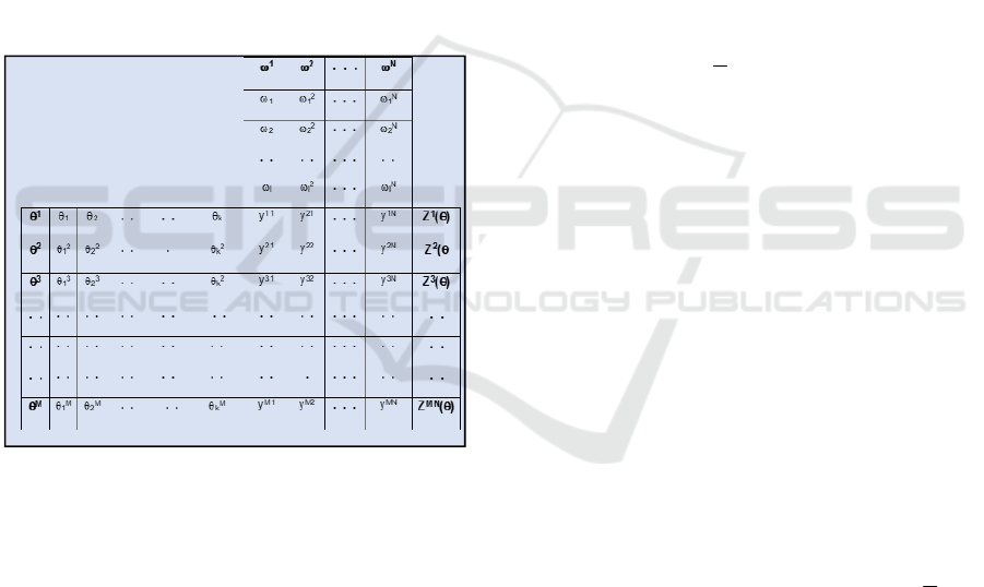
using a 2
3
full factorial design. The notation used in
this table is defined as follows:
Let Y represent a performance measure of interest
(e.g., throughput, flow time, machine utilization,
work-in-process).
Let y
IJ
represent a realization of this performance
measure for system configuration or system design I
=1, 2,…M, and noise set J = 1,2,…, N.
Let
θ
i
I
represent the setting of the i
th
controllable
variable (i= 1, 2,…, k) for system configuration I
(e.g., number of AGVs, AGV speed, AGV
dispatching rule, machine queue discipline in force).
Let
ω
J
represent a set of noise conditions, J=1,2,
...N
Let
ω
j
J
represent the j
th
noise variable setting (j =
1, 2, …, l) for noise condition J (e.g., machine mean
time between failure, mean time to repair, mean
interarrival time).
Table 4: Data Collection Plan.
Let Z
I
( θ ) represent a performance statistic for
each design configuration (e.g., mean or variance of
a performance measure such as throughput, flow
time, machine utilization, work-in-process).
Z
I
( θ ) is a function or functions of all of the data
that have been selected by the simulation analyst to
examine one or more aspects of the performance of
system configuration i over the noise conditions. By
examining different choices for Z, the experimenter
can examine various system performance aspects.
This research focuses on examining the mean
system performance, the system variance with respect
to noise (Var
(wrtn)
), the maximum and minimum
system performance. Therefore, Z
I
( θ ) may represent
a vector of values such as the row average, the row
variance, and the row maximum or row minimum.
This simulation data collection plan described
above represents a departure from the procedures
discussed in the literature of experiments. The
associated design of experiments strategy for robust
design can facilitate detailed analysis. A robust
system design is, then, one that performs desirably
and consistently under all the noise conditions
represented in the simulation experiments.
5 VARIANCES, MAIN AND
INTERACATION FACTORS
A well-planned experiment makes it simple to
subsequently analyze and predict the improved
(optimal) parameter settings. In this study, for each of
the simulated design configurations i, eight
measurements (over the set of noise factor
combinations) were taken for each performance
measure of interest, and then, averaged across the
replications to obtain
i
y
for each i
th
row of the inner
array. Sixteen design configurations and five center-
points (for a total of 21) designs were simulated over
a set of eight noise factor combinations, leading to a
total of 21 x 8 =128 simulation runs. The results of
these various simulation experiments, too large to be
displayed in this paper, but available upon request,
were subsequently averaged up across the three
replications.
This research intends to minimize the variances of
the performance measures with respect to the noise
factors for each run.
5.1 Determination of Main Effects on
Means and Variances
The objective is to make the variances of the
responses (performance measures) as small as
possible while bringing the means to their optimum
settings, i.e., minimum MFT and maximum for the
TR. The study then computes the values of
i
y
and
log
σ
2
(wrtnf)i
at each design configuration.
Subsequently, the effects of each control factor on
the overall mean and the variance (or log
σ
2
wrtnf
) are
calculated using the normal probability method. The
same procedure is applied to the complete set of
controllable factors to assess the effects on the means
of Throughput Rate (TR), Mean Flow Time (MFT),
Work-in-Process (WIP), and Utilization (UT).
ICORES 2024 - 13th International Conference on Operations Research and Enterprise Systems
312

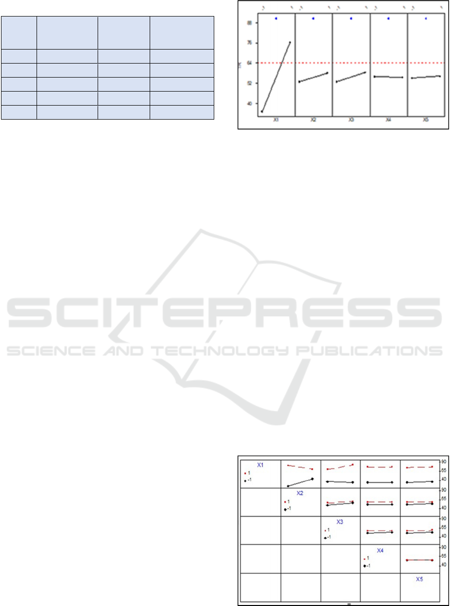
Table 5: Effects of Control Factors MFT Variance.
Control
Factors
Effect on MFT
log σ
2
wrtnf
Level (+1)
Effect on log
MFT σ
2
wrtnf at
Level (-1)
Absolute Value
Difference
X
1
1.6159 1.657502 0.04155
X
2
1.6081 1.558286 0.04982
X
3
1.4921 1.781325 0.28920
X
4
1.6338 1.639566 0.00568
X
5
1.6032 1.670230 0.06701
The results, not all displayed in this paper, are
available upon request. Then each controllable factor
is tested at two levels and the magnitude of its effect
on the mean measured.
Table 5 displays the effects of controllable factors
on the MFT mean, just as an illustrative example.
Analysis of the results in Table 5 reveals that X
3
(queue discipline) has the most significant effect on
the MFT variability as highlighted in bold, while the
exam of other results shows that X
1
(number of
AGVs) has the most significant effect not only on the
MFT mean but as well as on the TR variability and
mean. These results agree with previous findings
Bardhan and Tshibangu, 2002, Tshibangu 2003).
Subsequently, the effect at high level is compared
to the effect at low level, and the better setting of each
control parameter is that gives the smaller average
value of log
σ
2
wrtnf
. Results indicate that factor X
1
(the
number of AGVs), when set at its high level, has the
most significant effect on the mean value of MFT.
Other results, not displayed here, but available upon
request, indicate a high impact of X
1
(the number of
AGVs) on TR.
Once identified, these significant factors for MFT
and TR will be set at the settings (levels) that
minimize log
σ
2
wrtnf
., i.e., X
1
and X
3
at high settings,
and these, implemented. Note that a visual summary
of the magnitude of each control factor’s effect can
also be used for analysis of various effects.
The relative importance of different main effects
of control factors on the means and variances have
been derived. Figure 2 displays a visual
representation of the main effect on TR means for
illustration purpose. Other graphs exist for the effects
on variances and means of all other controllable
factors. A quick glance at Figure 2 and others, not
displayed here, reveals on one side, that control factor
X
1
(fleet size) is a critical factor because it has a
significant effect on the TR and MFT means and on
TR Variance. On the other side, Factor X
3
(queue
discipline) has the biggest effect on MFT variance.
This agrees with the analytical results (Tshibangu
2003).
Figure 2: Main Effect Plot (data means) for TR.
5.2 Determination of 2-Way
Interaction Effects
Effects due to interaction between factors are
important in selecting an experimental design,
because underestimating these effects may lead to
incorrect conclusions whereas overestimating them
may unnecessarily increase the experimental design
size (Tshibangu 2003).
This research uses a resolution V design to allow
an estimation of effects of two-way interactions. The
effects of interactions between factors are determined
using a Minitab software package for the estimation
of main effects. As an example, and for illustration
purposes, Figure 3 displays a 2-way interaction
between mean values control factor TR.
To be certain that the samples collected through
simulation and robust design of experiments
approaches are statistically valid, all the necessary
hypothesis and normal probability tests have been
conducted at 95% confidence level.
Normal probability plots are useful in assessing
the significance of effects from a fractional factorial,
especially when several effects are to be estimated
(Montgomery 2013).
Figure 3: Interaction Plots (data means) for TR.
An Alternative Robust Design to Assist a Single-Objective Performance Optimization: Simulation Analysis of a Flexible Manufacturing
System
313

6 OPTIMIZATION SCHEME
IMPLEMENTATION
In this section, a unique optimization procedure is
developed and presented. The developed
optimization procedure represents a departure from
other approaches reported in the literature in the sense
that this procedure is the first to include the effects of
two-way interaction between controllable factors.
The approach is inspired and motivated by Taguchi’s
strategy for improving product and/or process quality
in manufacturing.
6.1 Four-Step Single-Response
Optimization Approach for Robust
Design
Because flexible manufacturing systems and any
other process-oriented systems are subject to various
uncontrollable factors that may adversely affect their
performance, a robust design of such systems is
crucial and unavoidable. The author has developed a
four-step optimization procedure to be used
simultaneously with the robust design as first step of
the optimization scheme as proposed in this study:
Let
i
y
represent the average performance measure
across all the set of noise factors combination,
averaged across all the simulation replications for each
treatment combination (or design configuration) i.
Let log σ
2
wrtnf(i)
be the associated logarithm of the
variance with respect to noise for that treatment i.
Kacker and Shoemaker, 1986 recommend using the
logarithm of the variance to improve statistical
properties of the analysis, and to employ the “effects”
values and/or graphs in association with normal
probability plots and or ANOVA procedures to
identify and partition the following three categories
of control factor vectors:
Under the assumption that we have partitioned
three categories of control vectors as non-empty sets
X
v
T
containing the factors that have a significant effect
on the variances, X
m
T
containing factors significant on
the means (and their interactions), and X
0
T
as the set of
the factors that affect neither the mean nor the variance,
respectively, then a four-step empirical optimization
procedure may be implemented as follows:
Step 1
Identify the vector X
v
T
and adjust the controllable
factors members of this set to their values that
minimize
σ
2
wrtnf
.
of the performance measure y.
Step 2
Identify vector (X
m
T
)
1
of factors having a
significant effect on the mean
y
and set the
controllable factors members of this set to their
level values that optimize the mean
y
of the
objective performance y. Also, identify (X
m
T
)
2
vector of factors having a significant effect on
mean
y
and on the variance σ
2
wrtnf
simultaneously and set the factor members of this
set to their level values that optimize the mean
y
if this setting does not act in opposition with the
minimization of the variance. Otherwise, find a
compromise between minimizing the variance
and optimizing the mean as suggested in Step 4
where the final setting is to be decided.
Step 3
Identify the vector X
0
T
and set the control factors
members of this set to the values of their
interaction with members of vector X
v
T
that
minimize the variance or log
σ
2
wrtnf
or the values
of their interaction with members of X
m
T
that
optimize the mean
y
. Otherwise, set the factors at
their economic settings.
Step 4
Conduct a small follow-up experiment to find the
trade-off between members of (X
m
T
)
2
B
containing
factors with effects on variance and mean acting
in opposition and or the overall economical
settings. A suggestion from this study is that in
finding the overall economical setting, the step
involves only those factors that have the greatest
effect on either the variance
σ
2
wrtnf
or the mean
y
.
6.2 Throughput Rate (TR) and Mean
Flow Time (MFT) Optimization
When applying the above-described procedure the
optima for TR (maximum) and MFT (minimum) are
found using the associated plots and tables, the
following result are obtained:
For Throughput Rate (TR)
X
v
T
: [X
1
(-1), X
2
(-1)], pending (X
1
and X
2
adjustment through follow-up and confirmatory
runs).
X
m
T
: [X
5
(-1)], confirmed.
X
0
T
: [X
4
(-1), X
5
(-1)], confirmed.
For Mean Flow Time (MFT)
X
v
T
: X
3
(+1), confirmed.
(X
m
T
): (X
m
T
)
1
: X
1
(+1), X
2
(+1)
(Xm
T
)
2
: (X
m
T
)
2
A
: X
3
(+1), confirmed.
(X
m
T
)
2
B
: φ
(X
0
T
): X
4
(-1), X
5
(-1), confirmed.
ICORES 2024 - 13th International Conference on Operations Research and Enterprise Systems
314

6.3 Follow-up and Confirmatory Runs
Follow-up and confirmatory experiments are then be
conducted under the above specified system
conditions. For each configuration tested, besides the
primary performance measures TR and/or MFT, other
performance measures such as machine utilization,
work-in-process (WIP), and AGV utilization are also
recorded for benchmarking purposes. The results of
the tuning and confirmatory runs at different settings
for TR and MFT are displayed in Table 11 and 12,
respectively.
At the completion follow-up/confirmatory, the
most optimal and robust design to be implemented
with respect to the performance measure of interest
TR (used here as an example) is highlighted in bold
in Table 6.
Table 6: TR Optimization follow-up/Confirmatory Runs
Under Various #AGVs (X
1
) & AGV Speed (X
2
).
7 RESULTS AND
COMPARATIVE ANALYSIS
In both TR and MFT cases, the results obtained are
compared with those generated by similar procedures,
such as Taguchi (using S/N ratio), Kacker and
Schoemaker (1986), Wild and Pignatiello (1996), and
Bulgak et al. (2000) approaches. Table 7 depicts one
of the primary performance measures of optimal
robust design configurations as achieved under
various approaches. The reader is referred to
Tshibangu 2003 for details and background about
each procedure.
TR optimal design yields the highest throughput
rate of (3000 parts/day), a fair machine utilization rate
of (89.73%), an acceptable WIP (81 parts/day) and a
relatively high AGV utilization (97.87%). Indices
100, 150, 200 refer to AGV speed in (ft/min). Using
the natural values, the optimum of MFT is achieved
with fleet of 6AGVs, at 200ft/min, SPT queue
discipline, FCFS AGV dispatching rule, and a buffer
capacity of 8 units, yielding MFT of 0.3666 min/part
in coded units, machine utilization of (86.5%), a
decent WIP of (77 parts/day) and an AGV utilization
rate of (90.19%).
8 CONCLUSIONS AND FUTURE
RESEARCH
The coronavirus crisis has dramatically increased risk
for every business, with many, experiencing shocks
in both supply and demand. Manufacturing plants are
at the center of that uncertainty, and their continued
operation through the crisis and beyond will depend
in large part on the organization’s ability to navigate
these wider risks (Vivek et. al. 2020).
In this study, a unique single-objective
optimization procedure is developed and presented.
Because of supply chain disruptions that have been
experienced in the manufacturing and production
industry, many organizations had to develop strategic
approaches for survival by focusing on few key
performance indicators, such as timely delivery of
manufactured goods, or solely on the volume of
products in need on the market.
Regardless of the selected KPI it was imperative
to be the best in the market segment. This study has
been motivated by the pandemic crisis to develop and
propose a robust single-objective optimization
procedure and apply it to a Flexible Manufacturing
System (FMS) that has been designed and analyzed
using a discrete-event simulation approach.
The developed approach is an approximation and
empirical procedure that takes advantage of a unique
robust design formulation to include the
consideration of the two-way interaction factor
effects. Although inspired and motivated by
Taguchi’s strategy for improving product and/or
process quality in manufacturing, the developed
procedure, however, the intentionally departs from
Taguchi’s and traditionally known approaches as it
avoids the criticisms and insufficiencies thereof.
Hence, a series of additional statistical tools is used to
assist the procedure. These include main and
interaction effects of control factors, t-test, ANOVA,
normal probability plots, etc.
As further research pathway, the optimal values
found in this single objective optimization procedure
could then be used as target value in any subsequent
multiple optimization scheme to be developed in
future research studies.
An Alternative Robust Design to Assist a Single-Objective Performance Optimization: Simulation Analysis of a Flexible Manufacturing
System
315

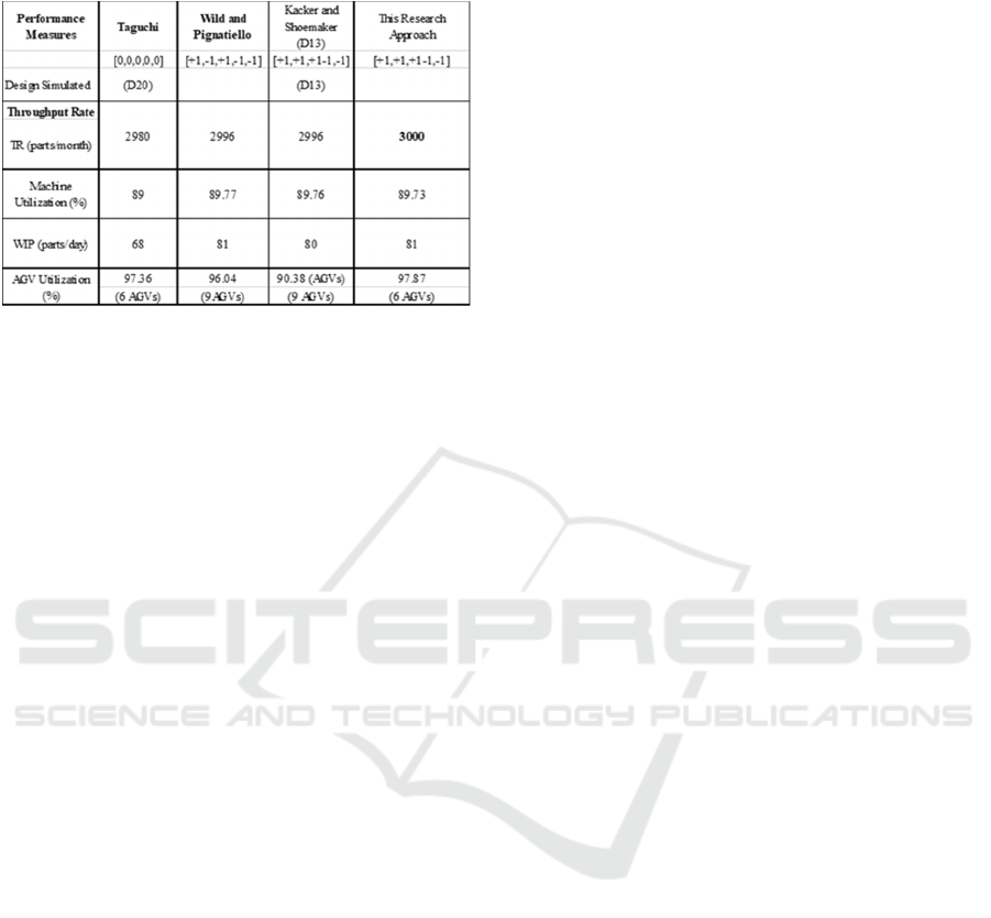
Table 7: Comparison Optimal TR as Realized under
Various Approaches.
The procedure is developed and applied to the
simulation outputs, focusing on optimizing TR (max)
and MFT (min). These performance measures have
been selected because they are extensively referred to
as primary KPIs in the literature. Follow
up/confirmatory runs are subsequently conducted as
sensitive analysis to fine-tune and validate the
settings initially uncovered through the first
approximation.
There are three areas of focus can help plant
managers and leaders navigate the transition from
initial crisis: (i) Protect the workforce: standardize
operating procedures and processes; (ii) Manage risks
to ensure business continuity: anticipate potential
changes and model the plant to react to fluctuations
to enable rapid, fact-based actions. (iii) Drive
productivity at a distance: Continue to effectively
manage performance at the plant while physical
distancing and remote working policies remain in
place.
As future research, the single-objective optimal
values can subsequently be used as targets for a more
advanced analytical multiple-objective optimization
scheme, using tools such as simulation metamodels.
In addition, the multiple objective-optimization could
include other KPIs such machine utilization, WIP,
and AGV utilization as primary metrics instead of
benchmarks or decision guides as used in this
research (Abdessalem et. al, 2022).
REFERENCES
Abdessalem et. al., 2022. Multi-Objective Design
Optimization of Flexible Manufacturing Systems Using
Design of Simulation Experiments: A Comparative
Study, Machines 2022, 10, 247.
Ball, P. and Love, D. (2009). Instructions in Certainty,
Institute of Industrial Technology, 29-33.
Bardhan, T. K, and Tshibangu W. M. A. 2003. Analysis of
an FMS with Considerations of Machine Reliability,
Proceedings of 8thAnnual IJIE Engineering Theory,
Applications and Practice, Las Vegas, Nevada.
Cappelli, A., Cini, E., (2020). Will the COVID-19
Pandemic Make us Reconsider the Relevance of Short
Food Supply Chains and Local Productions? Trends
Food Sci. Technol., doi: 10.1016/j.tifs.2020.03.041.
Cohen, M.J. (2020). Does the COVID-19 Outbreak Mark
the Onset of a Sustainable Consumption Transition?
Sustain. Sci. Pract. Policy,doi: 0.1080/15487733.20
20.174047.
Kacker, R. N., Shoemaker, A. C., Robust Design, 1986. A
Cost-Effective Method for Improving Manufacturing
Processes., AT&T Technical Journal, Volume 65, 51-84
Kleijnen, J. P. C., Design and Analysis of Simulations,
1977. Practical Statistical Techniques, SIMULATION,
Volume 28, no.3, 81-90.
Kumar, Aalok et al. (2020) COVID-19 impact on
Sustainable Production and Operations Management.
Sustainable Operations and Computers, Vol. 1, 1-7.
Montgomery, D. C., 2013, Design & Analysis of
Experiments, (8th Edition, NY: John Wiley & Sons Inc.
Park et al., 2001, FMS design Model with Multiple
Objectives Using Compromise Programming,
International journal of Production Research, Volume
39, no. 15, 3513-3528.
Ribeiro, J. L., and Elsayed, E. A., 1995. A Case Study on
Process Optimization Using the Gradient Loss
Function, International Journal of Production
Research, Volume 33, no. 12.
Taguchi, G., 1986. Introduction to Quality Engineering-
Designing Quality into Products and Processes, Asian
Productivity Organization, Tokyo.
Tshibangu W. M. A., 2005. A Framework for Designing a
Robust Material Handling Using Simulation and
Experimental Design, Proceedings of the 10th IJIE
Conference Florida.
Tshibangu, W. M. 2006, Robust Design of an FMS: S. M.
Proceedings of the GCMM, COPEC, Council of
Research in Education and Sciences November19-22,
Santos, Brazil.
Vivek, et al., 2020, Managing a manufacturing plant
through the corona virus crisis, McKinsey article, Apr
23.
Wild, R. H., and Pignatiello, J. J., Jr., 1991.An
Experimental Design Strategy for Designing Robust
Systems Using Discrete-Event Simulation,
SIMULATION, Volume 57, no.6, 358-368.
ICORES 2024 - 13th International Conference on Operations Research and Enterprise Systems
316