SIDAR: Synthetic Image Dataset for Alignment & Restoration

Monika Kwiatkowski

, Simon Matern

and Olaf Hellwich

Computer Vision & Remote Sensing, Technische Universit

at Berlin, Marchstr. 23, Berlin, Germany

Keywords:

Synthetic Dataset, Image Alignment, Homography Estimation, Dense Correspondences, Image Restoration,

Shadow Removal, Background Subtraction, Descriptor Learning.

Abstract:

In this paper, we present a synthetic dataset generation to create large-scale datasets for various image restora-

tion and registration tasks. Illumination changes, shadows, occlusions, and perspective distortions are added to

a given image using a 3D rendering pipeline. Each sequence contains the undistorted image, occlusion masks,

and homographies. Although we provide two speciﬁc datasets, the data generation itself can be customized

and used to generate an arbitrarily large dataset with an arbitrary combination of distortions. The datasets al-

low end-to-end training of deep learning methods for tasks such as image restoration, background subtraction,

image matching, and homography estimation. We evaluate multiple image restoration methods to reconstruct

the content from a sequence of distorted images. Additionally, a benchmark is provided that evaluates keypoint

detectors and image matching methods. Our evaluations show that even learned image descriptors struggle to

identify and match keypoints under varying lighting conditions.

1 INTRODUCTION

Many classical computer vision tasks deal with the

problem of image alignment and homography esti-

mation. This usually requires detecting sparse key-

points and computing correspondences across multi-

ple images. In recent years, increasingly more meth-

ods have been using neural networks for feature ex-

traction and matching keypoints (Sarlin et al., 2020;

DeTone et al., 2018). However, there still is a lack

of datasets that provide sufﬁcient data and variety to

train models. In order to train end-to-end image align-

ment models, large datasets of high-resolution im-

ages are necessary. Existing end-to-end deep learn-

ing methods, therefore, utilize datasets containing

sparse image patches (Balntas et al., 2017), dense

correspondences from structure-from-motion (SfM)

datasets (Li and Snavely, 2018; Schops et al., 2017)

or optical ﬂow datasets (Butler et al., 2012a). Image

patches only provide sparse correspondences between

images, SfM datasets often lack a variety of scenes,

and optical ﬂow data has a high correlation between

images with small displacements.

A synthetic data generation for image alignment

and restoration (SIDAR) is proposed. A planar ob-

https://orcid.org/0000-0001-9808-1133

https://orcid.org/0000-0003-3301-2203

https://orcid.org/0000-0002-2871-9266

ject is generated, and a texture is added to its surface

to simulate an artiﬁcial painting. Randomized geo-

metric objects, lights, and cameras are added to the

scene. By rendering these randomized scenes, chang-

ing illumination, specular highlights, occlusions, and

shadows are added to the original image. The data

generation uses images from the WikiArt dataset (Tan

et al., 2019) to create a large variety of content. How-

ever, the data generation can take any image dataset

as input. For each image, several distorted images

are created with corresponding occlusion masks and

pairwise homographies. The datasets can be used for

multiple objectives, such as homography estimation,

image restoration, dense image matching, and robust

feature learning. The rendering pipeline can be con-

ﬁgured to generate speciﬁc artifacts or any combina-

tion of them. It can be used as a data augmentation

to any existing datasets to further improve the perfor-

mance and robustness of existing methods.

Our dataset and rendering pipeline provide the fol-

lowing contribution:

• Data quantity: An arbitrary number of distortions

can be generated for each input image. Arbitrar-

ily, many scenes can be generated with an arbi-

trarily long image sequence each.

• Data variety: The input images and the image dis-

tortions can create a signiﬁcant variation in con-

tent and artifacts.

Kwiatkowski, M., Matern, S. and Hellwich, O.

SIDAR: Synthetic Image Dataset for Alignment & Restoration.

DOI: 10.5220/0012391400003660

Paper published under CC license (CC BY-NC-ND 4.0)

In Proceedings of the 19th International Joint Conference on Computer Vision, Imaging and Computer Graphics Theory and Applications (VISIGRAPP 2024) - Volume 3: VISAPP, pages

175-189

ISBN: 978-989-758-679-8; ISSN: 2184-4321

175

Figure 1: A visualization of the randomized rendering

pipeline in Blender. An image is added as texture to a

plane. Randomized cameras are positioned into the scene,

described by the white pyramids. The yellow rays describe

light sources, such as a spotlight and an area light. Geomet-

ric objects serve as occlusions and cast shadows onto the

plane.

• Customizability: The rendering pipeline can be

conﬁgured to control the amount and type of ar-

tifacts. For example, custom datasets can be cre-

ated that only contain shadows or occlusions.

In addition to the rendering pipeline itself, two

ﬁxed datasets are provided. One dataset is gener-

ated that only consists of image sequences from front-

parallel view with various distortions, such as chang-

ing illumination, shadows, and occlusions. Another

dataset is generated that, in addition to the aforemen-

tioned distortions, contains perspective distortions. In

order to reconstruct the underlying signal from a se-

quence of distortions, the information needs to be

aligned ﬁrst. Shadows and illumination change the

original signal but do not eradicate the information

completely. Occlusions cover the underlying con-

tent in parts of the image. However, for all these

cases, using additional images allows us to identify

and remove distortions using pixel-wise or patch-wise

comparisons along the temporal dimension. Perspec-

tive distortions create misalignment that makes recon-

struction more complicated. For this reason, we treat

misaligned images as a categorically different prob-

lem.

The following paragraphs discuss related datasets

and compare their advantages and shortcomings. The

rendering pipeline is described in detail. Finally,

we benchmark several methods for image registration

and image restoration. Our code is publicly avail-

able.

https://github.com/niika/SIDAR

2 RELATED WORK

In this section, we review some existing datasets and

compare them with our dataset. We discuss the appli-

cation of SIDAR.

2.1 Image Restoration & Background

Subtraction

Our data generation allows the creation of image se-

quences containing various distortions. In the case

of a static camera, this is similar to tasks such as

background subtraction or change detection. Exist-

ing datasets for background subtraction use videos of

static scenes (Vacavant et al., 2013; Goyette et al.,

2012; Jodoin et al., 2017; Toyama et al., 1999; Kalso-

tra and Arora, 2019). Each individual frame can con-

tain deviations from an ideal background image. The

variance can be due to changes in the background,

such as illumination changes, weather conditions, or

small movement of background objects. Addition-

ally, distortions can be caused by foreground objects

or camera noise. The goal is to extract a background

model of the scene, which can be further used for seg-

mentation into background and foreground.

When training deep learning models, one can

differentiate between scene-dependent models and

scene-independent models (Mandal and Vipparthi,

2021). Scene-dependent models learn a background

model on a speciﬁc scene and must generalize on

new images of the same scene. In contrast, scene-

independent models are evaluated on new scenes.

Many existing datasets, such as CDNet (Goyette

et al., 2012) or SBMNet(Jodoin et al., 2017), con-

tain many individual frames but only a few different

scenes. Training a model end-to-end on these datasets

allows the development of scene-dependent models,

but the low variation in scenes limits the generaliza-

tion across different backgrounds. Our data gener-

ation can create arbitrarily many variations within a

speciﬁc scene and across different scenes. This can be

useful to train and evaluate scene-independent mod-

els. Compared to video sequences, SIDAR has much

more variation between each image, and there is no

correlation between each frame.

The proposed SIDAR dataset can be customized

to generate speciﬁc artifacts, such as changes in illu-

mination, occlusions, and shadows. It can also cre-

ate any combination of these artifacts. One can apply

our dataset to train models for various tasks, such as

detecting and removing shadows, specular highlights,

or occlusions. Existing datasets containing shadows

(Wang et al., 2017; Kligler et al., 2018; Qu et al.,

2017) or illumination changes (Butler et al., 2012b;

VISAPP 2024 - 19th International Conference on Computer Vision Theory and Applications

176

Roberts et al., 2021) often deal with each artifact in-

dividually and provide less control over their combi-

nations.

The main shortcoming of our dataset is that it is

limited to perspective distortion and relies on syn-

thetic data generation. Certain artifacts caused by

the scene’s geometry or noise in the image formation

from real cameras cannot be synthetically replicated.

2.2 Homography Estimation

Homography estimation describes a fundamental task

in computer vision. However, few datasets provide

enough ground truth homographies between image

pairs to train a deep-learning model. A common ap-

proach to generate labeled data is to use any image

dataset, such as MS COCO (Lin et al., 2014), and ap-

ply perspective distortion (Chang et al., 2017; DeTone

et al., 2016; Erlik Nowruzi et al., 2017). These meth-

ods do not introduce any additional challenges or ar-

tifacts. Other methods apply perspective distortion to

video sequences with static cameras (Le et al., 2020;

Cao et al., 2022). The video sequences introduce dy-

namic objects that can create outliers when computing

correspondences between images. In both cases, the

perspective distortion is rather simple and does not

follow a camera projection of a planar object.

Datasets that rely on structure-from-motion or oth-

erwise estimate homographies from natural images,

such as HPatches (Balntas et al., 2017), Oxford

Afﬁne (Mikolajczyk and Schmid, 2005) or Adelai-

deRMF(Wong et al., 2011) only provide enough im-

age data to train deep learning models on smaller im-

age patches for feature detection. NYU-VP and YUD+

use detected planar objects in 3D scenes (Kluger

et al., 2020) to develop a large dataset that is used

for self-supervised training. However, both NYU-

VP and YUD+ only provide sparse correspondences

of line segments. HEB is a large-scale homography

dataset that contains image pairs with correspond-

ing homographies extracted from landmark images

(Barath et al., 2023). However, the image pairs also

only contain sparse keypoint matches.

For all of these datasets, there is little variation

in scenes, and each individual image does not con-

tain many distortions. Additionally, SfM datasets rely

on existing keypoint detectors, such as SIFT. Training

image descriptors on these datasets could add a bias

caused by the original descriptors.

Our proposed SIDAR dataset overcomes these

shortcomings by generating strong distortions within

each scene. Homographies can be computed regard-

less of the complexity of the scene and the amount of

artifacts.

As described in section 3.3, a homography can be

computed between any image pair if the relative po-

sition of cameras and plane are known. Furthermore,

we provide homographies between all images. This

allows for benchmarks where the relative orientation

of all images can be jointly estimated under various

distortions. It is possible to evaluate Bundle Adjust-

ment methods, and it could enable the development

of trainable Bundle Adjustment methods (Lin et al.,

2021; Lindenberger et al., 2021). Figure 3.2 illus-

trates a perfectly aligned image sequence in the pres-

ence of strong image distortions.

2.3 Descriptor Learning & Dense

Correspondences

Keypoint detection and image descriptors are fun-

damental methods in many computer vision tasks.

Structure-from-motion and other photogrammetric

methods rely on point correspondences computed

from sparse keypoints (Hartley and Zisserman, 2003).

A requirement for local feature detectors is to iden-

tify the location of distinct image points and com-

pute a robust feature representation. The features

should be invariant to various distortions, such as

noise, changing illumination, scale, and perspective

distortions. Recent developments in feature detec-

tors use a data-driven approach to learn robust feature

representations with deep learning (Mishchuk et al.,

2017; DeTone et al., 2018; Shen et al., 2020). The

descriptors are either trained on sparse image corre-

spondences from structure-from-motion methods (Li

and Snavely, 2018) or by applying randomized per-

spective transformations on any image dataset, such

as MS COCO (Lin et al., 2014), as described in sec-

tion 2.2.

SIDAR provides the ground truth homographies

between image pairs with arbitrarily complex arti-

facts. The dataset allows explicitly adding illumina-

tion changes, shadows, specular highlights, and data

augmentations to train more robust descriptors. Since

dense correspondences and occlusion masks are pro-

vided for each pixel, image descriptors can be com-

puted and matched for any image point. This also

allows the training of dense image matching models

(Truong et al., 2020; Truong et al., 2021). Structure-

from-motion datasets (Li and Snavely, 2018; Schops

et al., 2017) also provide dense correspondences, but

they often contain a limited amount of scenes, distor-

tions, and only a few occlusions. By changing the

texture of the image plane, SIDAR adds an arbitrarily

large variety of patches and keypoints.

SIDAR: Synthetic Image Dataset for Alignment & Restoration

177

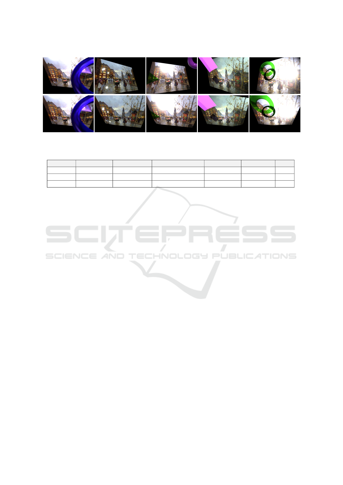
Figure 2: The ﬁrst row shows a sequence of images with perspective distortions. The second row shows the images warped

into the reference frame of the ﬁrst image using the precomputed homographies.

Table 1: Comparison of existing homography datasets and the proposed SIDAR dataset.

Dataset #Image pairs Camera poses Scene type Illumination Occlusions Real

HPatches 580 ✗ walls ✓ ✗ ✓

HEB 226 260 ✓ landmark photos ✓ ✗ ✓

SIDAR [55 000,∞) ✓ paintings / arbitrary ✓ ✓ ✗

3 RENDERING PIPELINE

Figure 1 illustrates the data generation process. We

use paintings from the Wiki Art dataset (Tan et al.,

2019) as our ground-truth labels. Any other image

dataset could also be used, but Wiki Art contains an

especially large variety of artworks from various pe-

riods and art styles. We believe that the diversity of

paintings makes the reconstruction more challenging

and reduces biases towards a speciﬁc type of image.

We take an image from the dataset and use it as a tex-

ture on a plane in 3D.

Furthermore, we generate geometric objects and

position them approximately in between the plane and

the camera’s positions. We utilize Blender’s ability to

apply different materials to textures. We apply ran-

domized materials to the image texture and occluding

objects. The appearance of an occluding object can

be diffuse, shiny, reﬂective, and transparent. The ma-

terial properties also change the effect lighting has on

the plane. It changes the appearance of specularities,

shadows, and overall brightness.

Finally, we iterate over the cameras and render the im-

ages. Blender’s physically-based path tracer, Cycles,

is used for rendering the ﬁnal image. Path tracing en-

ables more realistic effects compared to rasterization.

It allows the simulation of effects, such as reﬂections,

retractions, and soft shadows.

3.1 Virtual Painting

We ﬁrst generate a 2D image plane. The plane lies on

the xy-plane, i.e., the plane is described as:

0 · x + 0 · y + z = 0 (1)

The center of the plane also lies precisely in the ori-

gin (0,0,0). The plane is described by its four corner

points. Let w,h be the width and height of the plane,

then the corners are deﬁned as:





w/2

h/2









−w/2

h/2





, (2)





w/2

−h/2









−w/2

−h/2





(3)

We scale the plane along the x and y direction to ﬁt

the image’s aspect ratio. We apply the given image as

a texture to the plane.

3.2 Fronto-Parallel View

To render the scene, we add virtual cameras. We dif-

ferentiate between a camera that is aligned with the

painting’s plane and a setup that adds perspective dis-

tortions. To enforce a fronto-parallel view, we use a

single static camera that perfectly ﬁts the image plane.

The camera’s viewing direction is set perpendicular

to the image plane and centered on the image plane.

Our goal is to adjust the vertical and horizontal ﬁeld

VISAPP 2024 - 19th International Conference on Computer Vision Theory and Applications

178

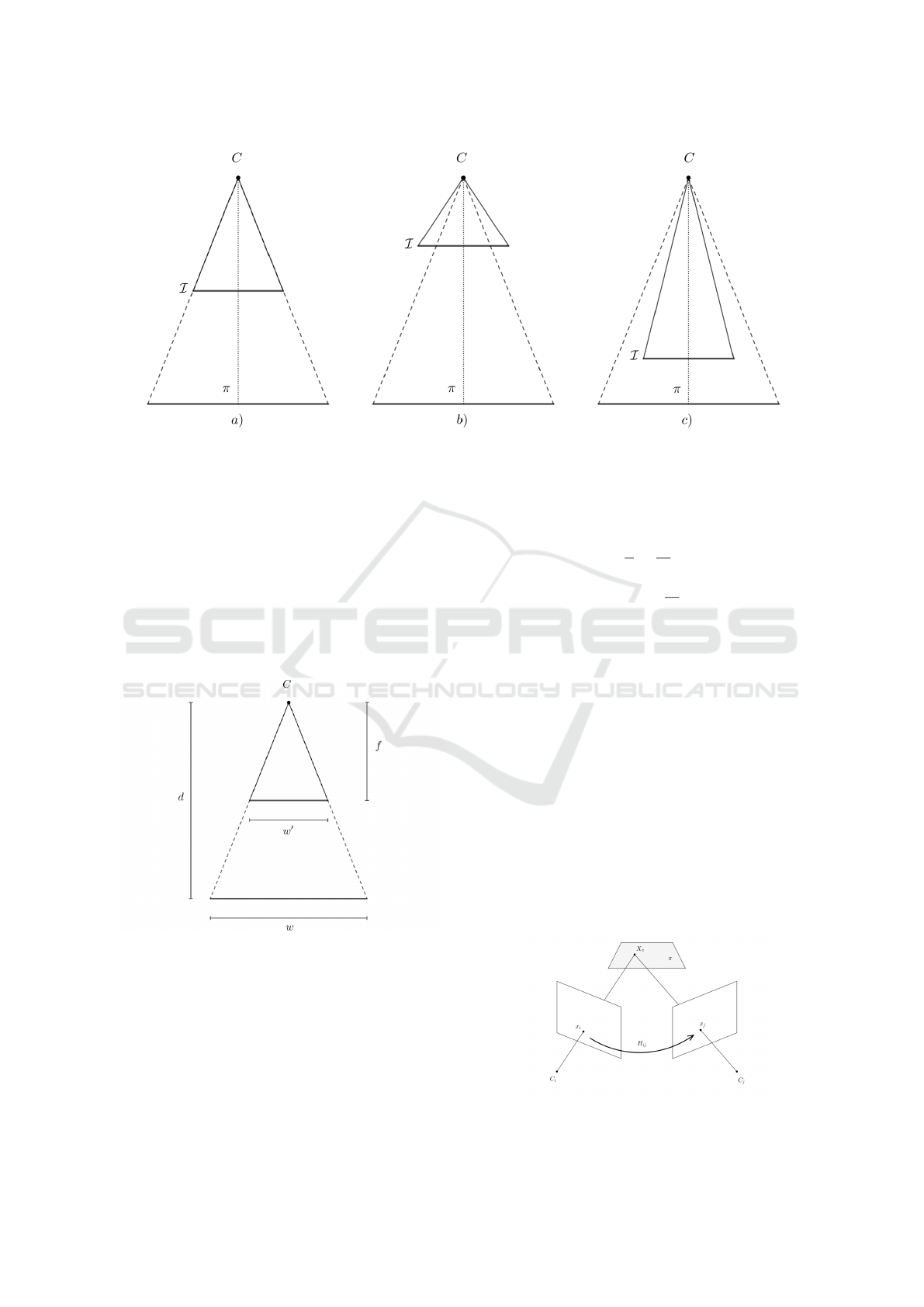
Figure 3: An Illustration of changing the principal distance between the projection center C and the image plane I . The

position of the plane π and the projection center are ﬁxed. In a) the image plane I captures all of the content from the painting

plane π and nothing more. In b), the camera’s ﬁeld of view is larger than the image plane. In c), the camera only sees parts of

the image.

of view such that only the image can be seen. Figure

3 illustrates this problem.

The camera’s projection center is set to the con-

stant C = (0,0, 10)

, and we also ﬁx the size of the

sensor. We set the resolution and aspect ratio of the

sensor equal to the painting’s resolution. As can be

seen in ﬁgure 3, the alignment only depends on the

principal distance.

Figure 4: Illustration of a camera sensor with width w

′

that

is aligned with the image with width w. The principal dis-

tance is given as f , and the distance between the camera and

image is given as d.

Let f be the principal distance, w the image width,

′

the sensor width, and d the distance between the

projection center and image as illustrated in ﬁgure 4.

The optimal f can be computed from the intercept

theorem:

′

(4)

⇔ f = d

′

(5)

3.3 Perspective Distortions

To create perspective distortions, we randomize the

generation of cameras by sampling from a range of

3D positions. The camera’s ﬁeld of view is also ran-

domly sampled to create varying zoom effects. This

also creates a variety of intrinsic camera parameters.

Additionally, we center the camera’s viewing direc-

tion into the image center. This is done to guarantee

that the image is seen by the camera. Otherwise, the

camera might only see empty space.

Since we project a planar object onto image

planes, all images are related by 2D homographies.

This relationship is illustrated in ﬁgure 5.

A point with pixel coordinates (x,y) in image i is

projected onto the coordinates (x

′

) in image j with

Figure 5: Illustration of a homography induced by a plane.

SIDAR: Synthetic Image Dataset for Alignment & Restoration

179

the homography H

i j





′





= H

i j









(6)

The homographies can be computed from the ori-

entation of the cameras and plane (Hartley and Zis-

serman, 2003):

i j

= K



R +

⃗

t⃗n



−1

(7)

Here R,

⃗

t describe the rotation matrix and translation

between cameras. K

and K

describe the calibration

matrices. ⃗n · X = d parameterizes the plane.

Alternatively, the homography can be computed from

point correspondences using the Direct Linear Trans-

form (Hartley and Zisserman, 2003). We decided to

use the Direct Linear Transform since it does not re-

quire traversing the scene graph and transforming the

objects relative to a new coordinate system. We com-

pute correspondences x

(k)

↔ x

(k)

by projecting the

corners of the painting into the images respectively:

(k)

= P

k = 1, ..,4 (8)

Here P

describes the projection matrix of the i − th

camera.

Unlike when working with real datasets, these

methods can always compute the corresponding ho-

mographies regardless of overlap and distortions.

Real datasets rely on more complicated photogram-

metric methods that try to ﬁnd point correspondences

between images and optimize the orientation of cam-

eras using bundle adjustment (Balntas et al., 2017;

Hartley and Zisserman, 2003; Li and Snavely, 2018).

Regardless of the complexity of the scene, the homo-

graphies can be precisely computed.

3.4 Illumination

We add varying illumination by randomizing the light

sources in the scene. The light is randomly sampled

from Blender’s predeﬁned light sources: spotlight,

point light, and area light. We randomize the inten-

sity and color of the light. This randomization can

create a large variety in the appearance of shadows,

specularities, and the overall color scheme of the im-

age.

The color is sampled using the HSV color space. Let

c = (H, S,V ) be the color of the light. We sample

c using H ∼ U[0, 1],S ∼ U[0,ε],V = 1. V is ﬁxed

because the intensity of the color is already affected

by the light source itself. The hue is completely ran-

domized to create random colors. However, the range

of the saturation is limited to a small ε to generate

lights that are closer to white. Having too high satu-

ration creates strong global illuminations changes that

make the reconstruction of the content’s original color

very ambiguous, while low saturation still introduces

enough variance in the appearance of the painting.

Furthermore, we set the orientation of the light such

that its direction is centered on the images. By de-

fault, Blender sets the orientation of the lights along

the z-axis.

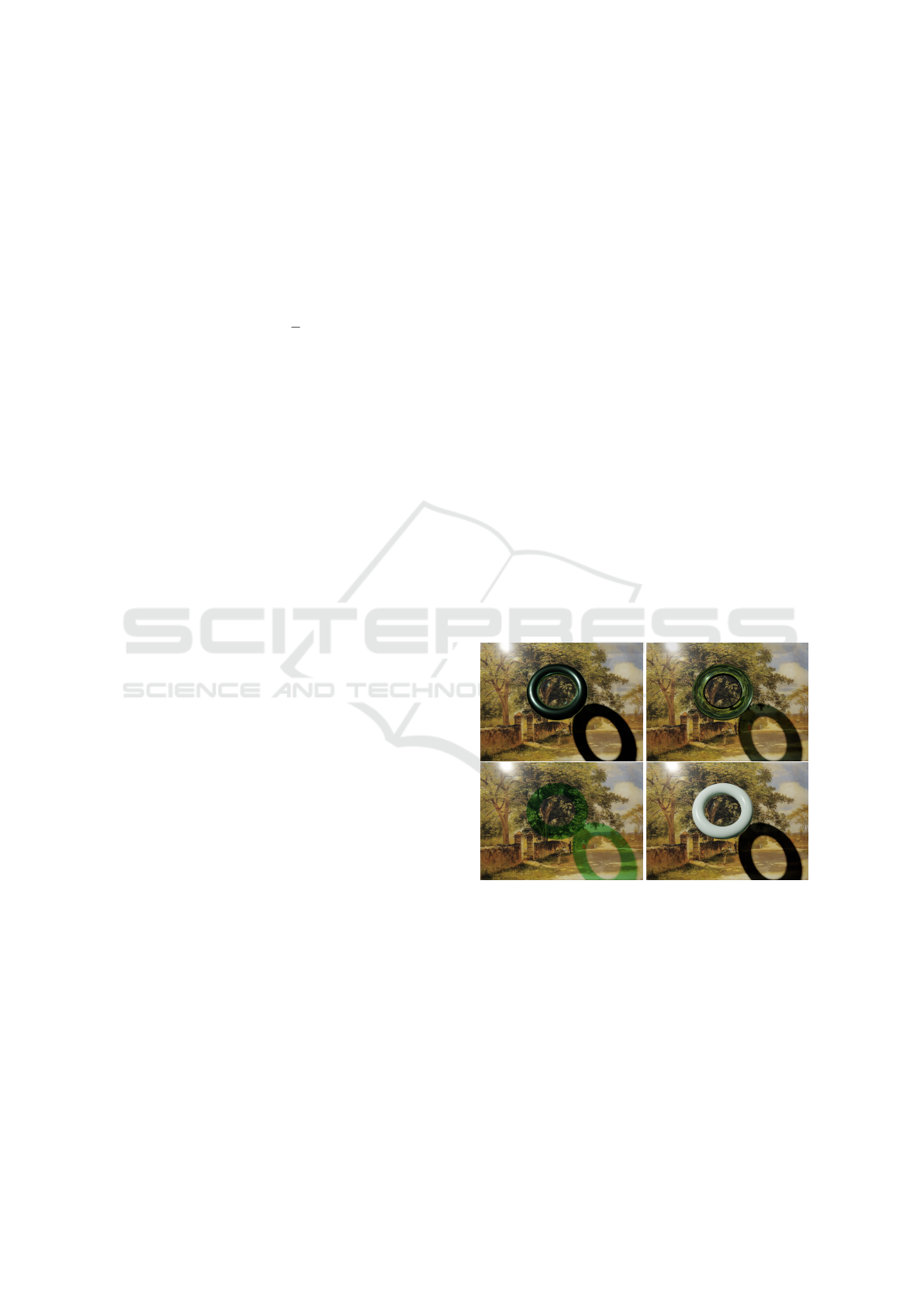
3.5 Occlusions & Shadows

Randomized geometric objects are added in the space

between light sources and the image plane. The

purpose of these objects is to create occlusions and

shadows. The objects obfuscate image content from

the cameras and block light from reaching the image

plane. The material of the object is also chosen from

Blender’s shaders. Depending on the material, light is

either completely blocked, refracted, or color-ﬁltered.

As can be seen in ﬁgure 6, the material affects the

appearance of the image content and casts a shadow.

Some materials create hard shadows and solid occlu-

sions, while others create softer shadows and even

change the shadow’s color. Transparent materials also

do not entirely obfuscate the image content.

Figure 6: A randomly generated torus under the same light-

ing conditions but with varying materials.

3.6 Rendering

After a scene is conﬁgured with randomized light-

ing, occlusions, and cameras, an image is rendered

using path tracing. Blender’s path tracer is used to

render the image from the perspective of a speciﬁc

camera. Path tracing allows the creation of more real-

istic shadows and lighting effects compared to rasteri-

zation; especially effects such as transparency, reﬂec-

tion, and refraction can be realistically modeled us-

VISAPP 2024 - 19th International Conference on Computer Vision Theory and Applications

180

ing path tracing by sampling light rays. Path tracing

simulates the physical image formation process much

closer than rasterization techniques. Rasterization re-

quires the use of various techniques, such as texture

maps and shadow maps, to approximate the same ef-

fects.The number of rays cast to estimate the light dis-

tribution of the scene and the resulting image can be

limited using a time constraint. A time limit is set to

balance the image quality and the amount of data that

can be efﬁciently generated. Figure 7 illustrates the

effect of rendering time on the resulting image. The

results do not differ too much. Shadows, illumination,

and occlusions are visualized correctly, even when us-

ing fewer rays. A low amount of sampling can create

aliasing effects, as can be seen on the glassy material.

In comparison, more sampling creates more realistic

effects.

Each rendered image describes a distorted data

point of the original image. Path tracing is also used

to generate the ground truth label. It is possible to

use the original image as a ground truth label. How-

ever, the rendering pipeline can create a bias and a

slight misalignment. For this reason, the label is cre-

ated under similar conditions as the distorted images

using ambient illumination without occlusion. A vir-

tual camera that is aligned with the image as described

in chapter 3.2 is used. The resulting image is free of

artifacts.

In order to differentiate between distorted parts of

the image (caused by lighting, shadows, and specu-

lar highlights) and occlusions, a segmentation mask is

computed that separates foreground and background

pixels. The mask should be aligned with the corre-

sponding camera. After rendering any scene, a corre-

sponding occlusion mask is rendered using the same

camera and geometric objects. For any given scene,

the plane’s material is changed to a diffuse black.

All objects are changed to a diffuse white material.

We also use ambient illumination. The segmentation

mask is rendered using regular rasterization. Figure

8 shows a mask generated from a given scene. The

resulting image is binary, with black pixels describ-

ing parts of the painting and white pixels describing

occlusions or background.

4 DATASETS

Using the rendering pipeline from chapter 3, we cre-

ate two datasets. By aligning the camera with the im-

age, we create a dataset of aligned sequences without

perspective distortion. Another dataset is created with

perspective distortions. In this chapter, we present the

two datasets and discuss some applications.

4.1 Fronto-Parallel Dataset

Figure 9 shows an example sequence of distorted im-

ages with the corresponding ground truth label. The

dataset contains ∼ 15000 image sequences each with

10 distorted images, ground-truth label and occlusion

masks. Since the image data is already aligned, it is

especially useful for image-to-image tasks, such as

image restoration, segmentation or autoencoders.

Image Restoration

Using the aligned dataset, a model can be trained to

remove artifacts from images. This can be done by

a sequential model that learns to aggregate informa-

tion from multiple images, such as Deep Sets (Za-

heer et al., 2017; Kwiatkowski and Hellwich, 2022)

Alternatively, a model can be trained to remove arti-

facts from single images, e.g., single-image shadow

removal (Qu et al., 2017). Existing methods often

deal with each type of artifact individually, whereas

this dataset allows combining multiple artifacts simul-

taneously. The data generation can be conﬁgured to

generate speciﬁc artifacts or combinations of them.

Using the occlusion mask, inpainting methods can be

trained to reconstruct the content of occluded regions.

Background Subtraction

The dataset can be used for background subtraction

tasks. The artifact-free image describes the under-

lying background, while lighting and occlusion cre-

ate distortions. A model can be trained to detect

occlusions and variations from the underlying back-

ground model. The generated occlusion masks can

be used for learning foreground-background segmen-

tation. Existing datasets consist of videos with a few

scenes, such as CDNet (Goyette et al., 2012). Al-

though the videos provide a lot of data, there is lit-

tle variation within each scene. Our dataset genera-

tion allows the creation of a large variety of different

scenes and also increases the variation within each

scene. This is useful to enable models to general-

ize over different backgrounds and make the back-

ground modeling more robust to changing lighting

conditions.

Representation Learning

Data augmentations, such as noise, blurring, random

cropping, and geometric transformations, are used to

create more robust representation learning or self-

supervised training (Chen et al., 2020; Bansal et al.,

2022). Using our dataset, a representation can be

learned that is invariant to illumination and occlu-

sions. Alternatively, a representation can be learned

SIDAR: Synthetic Image Dataset for Alignment & Restoration

181

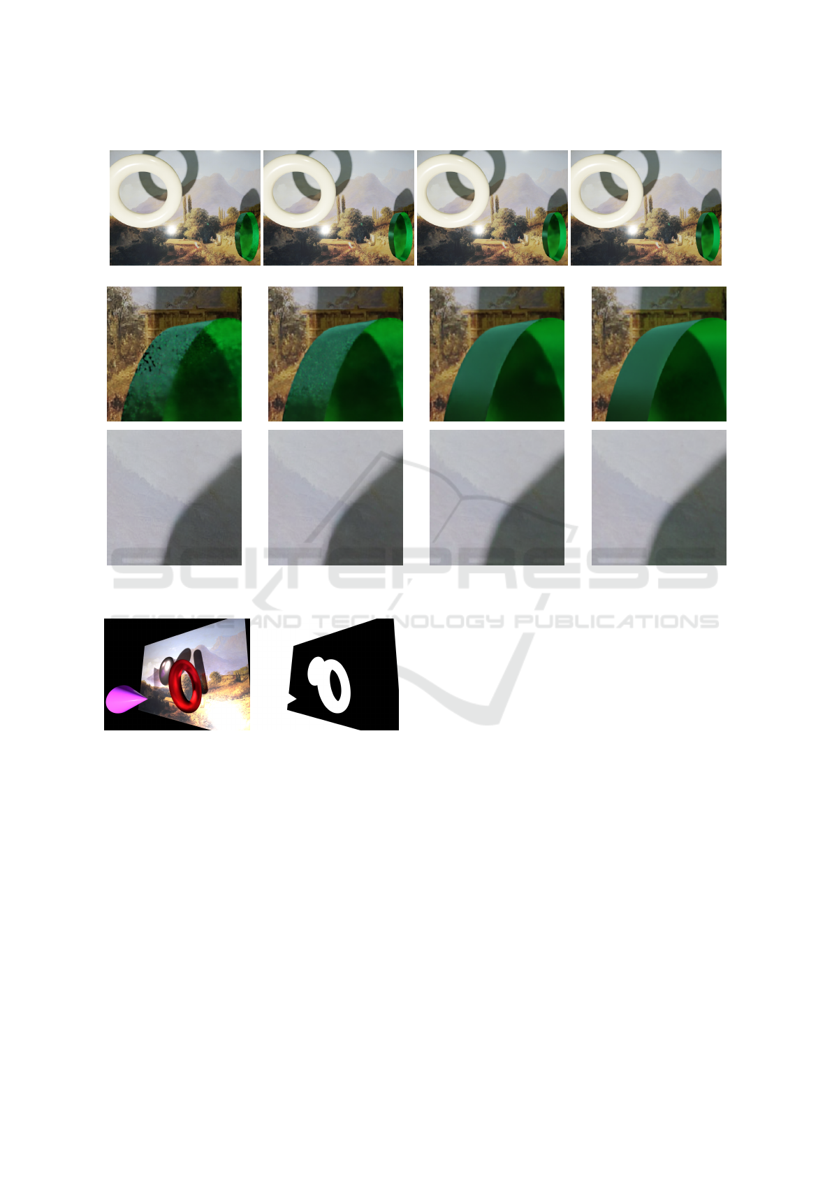
(a) 0.1s (b) 1s (c) 10s

(d) 5min

Figure 7: The images show the same scene rendered with different time limits. The ﬁrst row shows the whole image, while

the second and third rows show speciﬁc parts of the image.

Figure 8: The left image shows a randomized scene. The

right image shows the same scene after changing the plane

to a diffuse black and changing all geometric objects to a

diffuse white color. The rendered image is binary.

that disentangles the image content from lighting,

shadows, occlusions, etc.

4.2 Misaligned Dataset

In addition to the aligned dataset, we generate images

with perspective distortions. For each randomly gen-

erated camera, we render an image. In order to evalu-

ate the image alignment with reconstruction, we also

generate a single ground truth image as described in

section 3.2 under ambient lighting conditions. Figure

10 shows a sequence of distorted images. The last

image contains no distortions and is aligned with the

camera’s ﬁeld of view. We generate a dataset with

1000 sequences each containing 10 distorted images,

ground-truth label, segmentation masks. For each im-

age pair (I

, I

), the corresponding homography H

i j

is computed using DLT. The dataset contains 110000

homographies or 55000 if you exclude the inverse

mapping for each image pair.

It is possible to warp the image I

: R

7→ R

into the

reference frame of any other image I

: R

7→ R

us-

ing the warp function described by the homography

i j

: R

7→ R

i j

(x) = H

i j

x. The warped image

is calculated as:

(x) = I

−1

i j

(x)).

Figure 2 shows a sequence of images under perspec-

tive distortion. Using the estimated homographies, all

images can be aligned with the ﬁrst image.

The dataset containing perspective distortions ex-

tends all tasks mentioned in section 4.1, but it also

creates new challenges and applications. The follow-

ing chapters discuss some potential applications of

our dataset.

VISAPP 2024 - 19th International Conference on Computer Vision Theory and Applications

182

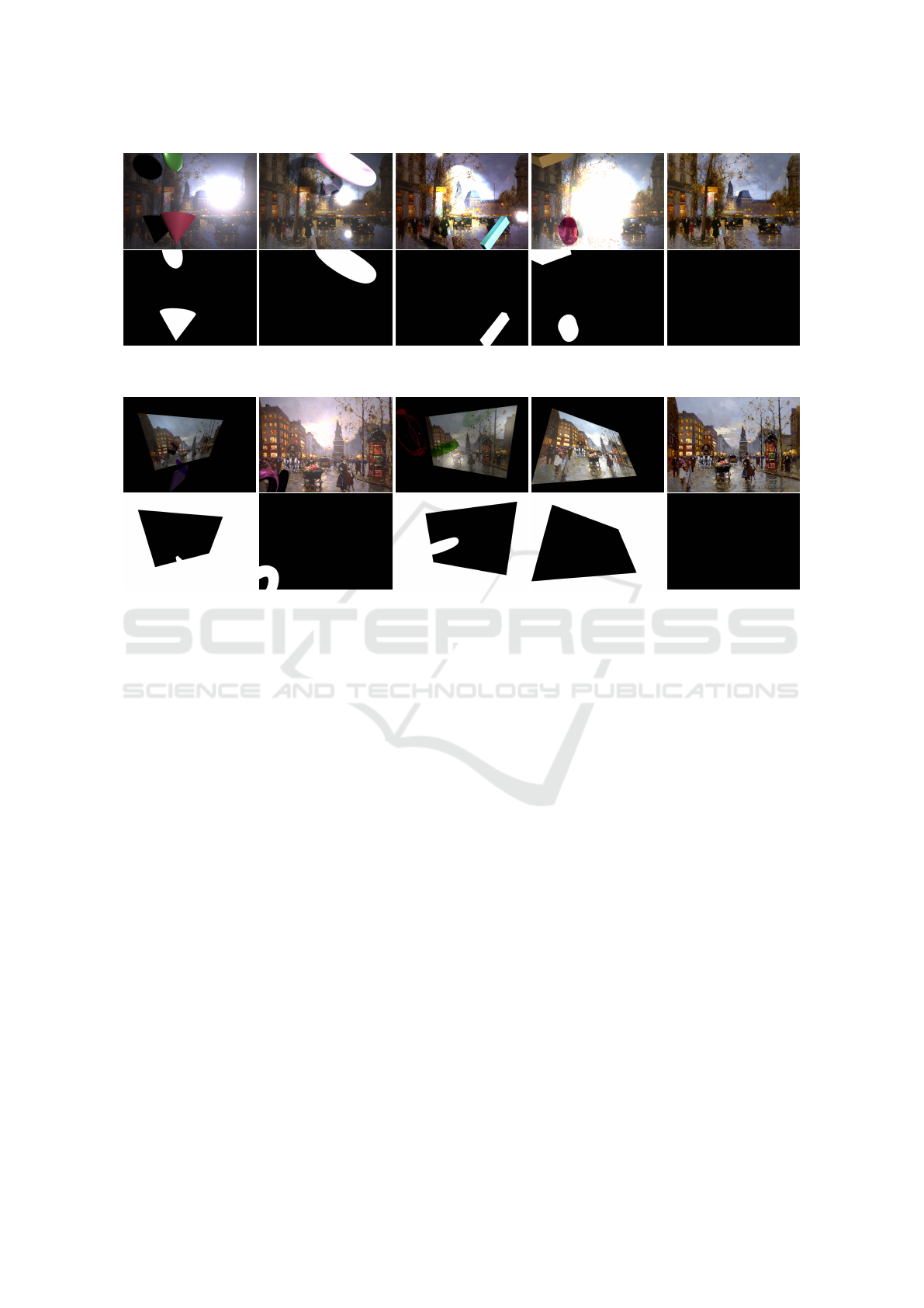
Figure 9: The top row shows four generated images without perspective distortions and with the corresponding label. The

bottom row shows the occlusion mask for each image.

Figure 10: The top row shows four generated images with perspective distortions and the corresponding label. The bottom

row shows the occlusion mask for each image.

Homography Estimation

Our dataset provides ground-truth homographies for

any image pair within a sequence, making it possi-

ble to train and evaluate deep homography estima-

tion methods. Let I

and I

be two images, let H

i j

their corresponding perspective transformation, and

let f

) ∈ R

be a deep learning model that esti-

mates a homography from two images. The learning

objective can be described by a regression problem:

i j

:= f

)

The homography parameters can be directly esti-

mated from two images.

Bundle Adjustment

Many existing homography estimation methods com-

pute the alignment from image pairs only. This can

be extended to sets of images. The problem can

be described as a bundle adjustment problem. The

SIDAR dataset can be used for neural bundle adjust-

ment methods, such as BARF (Lin et al., 2021). It

could be possible to learn neural priors for bundle ad-

justment. Larger image sets also enforce more con-

sistency across images compared to image pairs.

Descriptor Learning

Given the correspondences between images, local de-

scriptors can be learned. Correspondences exist even

under very strong distortions, which allows the de-

velopment of descriptors that are invariant or equiv-

ariant to the given perturbations. The methodology

of HPatches (Balntas et al., 2017) could also be ex-

tended to the SIDAR dataset to add more variety in

image patches.

Dense Correspondences

SIDAR also provides dense correspondences between

each image point with high accuracy and outlier

masking. Correspondences can be estimated not only

for sparse keypoints but for every pixel with a sub-

pixel accuracy. The neighborhood of points remains

mostly unchanged under perspective distortions. This

puts additional constraints on image-matching tasks.

The occlusion masks also provide regions of out-

liers, while the other distortions can add robustness

to image descriptors. Image matching models can be

trained to densely detect image regions under various

perturbations and also detect outliers as points with

no matches.

SIDAR: Synthetic Image Dataset for Alignment & Restoration

183

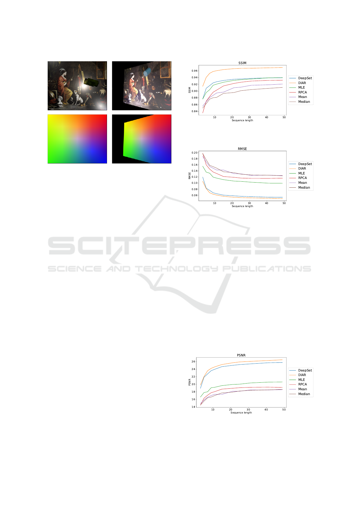
Figure 11: A visualization of dense correspondences be-

tween two images.

5 EXPERIMENTS

We study the performance of image alignment and

image restoration methods in the presence of signif-

icant distortions.

5.1 Image Restoration

Let D = {x

,· ·· ,x

} be a set containing distorted im-

ages. We compare several image restoration tech-

niques that involve reconstructing an image from dis-

torted image sequences. We use pixel-wise statisti-

cal methods, such as mean and median. Additionally,

we evaluate Robust PCA (Cand

es et al., 2011; Bouw-

mans et al., 2018), which decomposes the data matrix

M = [vec(x

),··· ,vec(x

)], that contains the vector-

ized images, as:

M = L + S

where L is a low-rank matrix and S is a sparse ma-

trix. RPCA assumes that distortions appear sparsely

described by the matrix S, whereas the content is very

similar in each image, resulting in a low-rank data ma-

trix L.

Furthermore, we use a maximum likelihood estima-

tion (MLE) for intrinsic image decomposition (Weiss,

2001). MLE assumes that image gradients approx-

imately follow a Laplace distribution. Under these

assumptions, the optimal image is reconstructed from

the median of the gradients.

In addition to the unsupervised methods, we

also train two models on our dataset. We use

Deep Sets (Kwiatkowski and Hellwich, 2022) and

DIAR(Kwiatkowski et al., 2022). We follow the orig-

inal implementations, but we removed any downsam-

pling layers. This led to a signiﬁcant improvement in

Figure 12: Comparison of image restoration methods using

SSIM with different sequence lengths.

Figure 13: Comparison of image restoration methods using

RMSE with different sequence lengths.

the cost of higher memory consumption. Both archi-

tectures use convolutional residual blocks. Deep Sets

apply average pooling over the sequential dimension,

whereas DIAR uses Swin-Transformers to aggregate

spatio-temporal features. Both models were trained

on a ﬁxed sequence length of 10 images.

Our evaluation set contains 100 sequences with 50

images each. As evaluation metrics, we use Struc-

tural Similarity Index Measure (SSIM), Root Mean

Squared Error (RMSE), and Peak signal-to-noise ra-

tio (PSNR). We evaluate each method on various se-

quence lengths. Figures 12,13 and 14 show the re-

sults.

The evaluations conﬁrm that the supervised meth-

ods have an overall superior performance. The graphs

show that all methods improve with increasing im-

age sequences. Even the supervised models general-

Figure 14: Comparison of image restoration methods using

PSNR with different sequence lengths.

VISAPP 2024 - 19th International Conference on Computer Vision Theory and Applications

184

ize well beyond their training length. DIAR has the

overall best performance. The spatio-temporal atten-

tion of the 3D-Swin-Transformer outperforms aver-

age pooling. Figure 15 shows an example sequence

with corresponding outputs and metrics.

5.2 Image Alignment

In order to evaluate image alignment methods, we

generate 1000 image sequences containing perspec-

tive distortions. Each sequence contains the orig-

inal image and ten distortions. This also results

in 55 homographies for each image sequence. We

use the available keypoint detectors and matchers

provided by OpenCV (Bradski, 2000) and Kornia

(Riba et al., 2020) for benchmarking. This includes

the unsupervised methods SIFT (Lowe, 1999), ORB

(Rublee et al., 2011), AKAZE, and BRISK (Tareen

and Saleem, 2018) and supervised methods LoFTR

(Sun et al., 2021), Superglue (Sarlin et al., 2020), and

AffNet-HardNet (Dmytro Mishkin, 2018). LoFTR

has weights for indoor scenes (LoFTR-i) and an out-

door scenes (LoFTR-o). Kornia also provides an im-

plementation of SIFT, denoted as SIFT-Kornia. For

each image pair, we detect and match keypoints.

Then, we compute the homography using RANSAC.

We evaluate the estimation of the homography by

computing the mean corner error (MCE):

MCE(H,H

′

) =

∑

i=1

∥Hx

− H

′

∥

where x

describes the corners of the image. Figure

17 shows the percentage of estimated homographies

below a given MCE. The results show that SIFT and

LoFTR consistently have better results depending on

the threshold. However, both are only able to ﬁnd ho-

mographies in ∼ 50% of all cases. We did not visual-

ize larger MCE values since larger errors indicate in-

correct homographies, which do not provide a mean-

ingful numeric value. This shows that keypoint de-

tectors and image descriptors struggle with the given

distortions.

Furthermore, we evaluate the individual matches x ↔

′

by computing the reprojection error:

L(x,x

′

) = ∥Hx

− x

′

∥

The error is measured in pixels. We compute the num-

ber of inliers based on the thresholds t ∈ {0.1, 1,10}.

Figure 16 shows the distribution of inliers for each

method. The results show that SIFT has the most re-

sults with subpixel accuracy. For larger thresholds,

the supervised methods provide much more matches

compared to SIFT and other unsupervised methods.

LoFTR-o has signiﬁcantly the most matches.

The benchmarks show that existing image match-

ing techniques struggle with changing illumination.

Since we did not ﬁnetune the supervised models,

the models might be biased towards keypoints from

SfM datasets. In future work we would like to ﬁne-

tune image matchers and keypoint detectors, such as

Superpoint, SuperGlue and LoFTR on our dataset.

Speciﬁcally, we believe one can combine the tech-

nique of Homographic Adaption (DeTone et al.,

2018) with our dataset, since Homographic Adap-

tion originally uses self-supervised training with triv-

ial perspective data augmentations. Furthermore, in

future work it should be possible to extend the bench-

marks and trainable methods to include joint match-

ing of the whole sequence instead of image pairs.

6 CONCLUSION

In this work, we propose a data generation with a cor-

responding datasets based on 3D rendering that intro-

duces various disturbances, such as shadows, illumi-

nation changes, specular highlights, occlusions, and

perspective distortions, to any given input image. Al-

though it is a synthetic dataset, the data augmenta-

tions are not trivial, and they are customizable. To the

best of our knowledge, we provide the ﬁrst large-scale

dataset containing ground-truth homographies with

dense image correspondences, which does not con-

sist of trivial perspective distortions. Our rendering

pipeline allows us to both generate new datasets and

augment existing data. We discuss several possible

applications. We discuss a range of computer vision

applications for which this dataset can be used. It can

contribute to the training of end-to-end deep learn-

ing models that solve image alignment and restoration

tasks such as deep homography estimation, dense im-

age matching, descriptor learning, 2D bundle adjust-

ment, inpainting, shadow removal, denoising, content

retrieval, and background subtraction.

The limitation of most synthetic datasets lies in

their deviation from real data. This can result in bi-

ased models and limit generalization. Compared to

existing augmentation methods that apply random-

ized homographies (DeTone et al., 2018) to images,

SIDAR adds additional complexity. Adding illumina-

tion changes, shadows, and occlusions can be espe-

cially helpful in improving the robustness of learned

descriptors and feature matching.

Future work could focus on developing bench-

marks to provide speciﬁc evaluation metrics for the

discussed tasks and compare the generalization across

different datasets. Additionally, future work could

further improve the realism of the data generation and

SIDAR: Synthetic Image Dataset for Alignment & Restoration

185

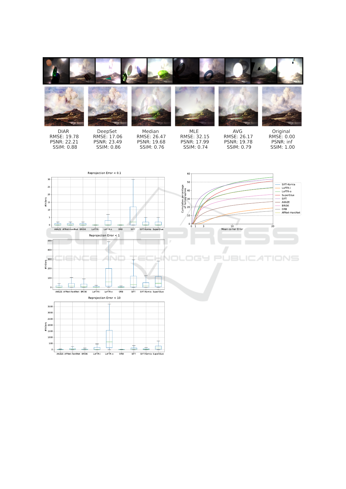
Figure 15: An overview of image restoration methods with corresponding image metrics. The ﬁrst row shows the input

sequence. The bottom row shows the reconstructed image by method.

Figure 16: The box plots show the number of inliers based

on different thresholds of the reprojection error.

add new data modalities, such as videos. The data

generation can be adapted to include other distortions,

such as reﬂective surfaces, translucent occlusions, or

camera lens distortions. Many of these effects are

common artifacts in real imaging systems, but it is

difﬁcult to create large-scale datasets for these cases.

Figure 17: The graphs show the cumulative percentage of

image pairs below a given Mean Corner Error.

Our data generation can provide an effective way to

approximate these artifacts and provide a large-scale

dataset for training and evaluation. It can serve as a

baseline to study these effects in a more controlled

environment.

REFERENCES

Balntas, V., Lenc, K., Vedaldi, A., and Mikolajczyk, K.

(2017). Hpatches: A benchmark and evaluation of

handcrafted and learned local descriptors. In CVPR.

Bansal, A., Borgnia, E., Chu, H.-M., Li, J. S., Kazemi, H.,

Huang, F., Goldblum, M., Geiping, J., and Goldstein,

T. (2022). Cold diffusion: Inverting arbitrary image

transforms without noise.

Barath, D., Mishkin, D., Polic, M., F

orstner, W., and Matas,

J. (2023). A large-scale homography benchmark. In

Proceedings of the IEEE/CVF Conference on Com-

puter Vision and Pattern Recognition, pages 21360–

21370.

Bouwmans, T., Javed, S., Zhang, H., Lin, Z., and Otazo,

R. (2018). On the applications of robust pca in im-

age and video processing. Proceedings of the IEEE,

106(8):1427–1457.

VISAPP 2024 - 19th International Conference on Computer Vision Theory and Applications

186

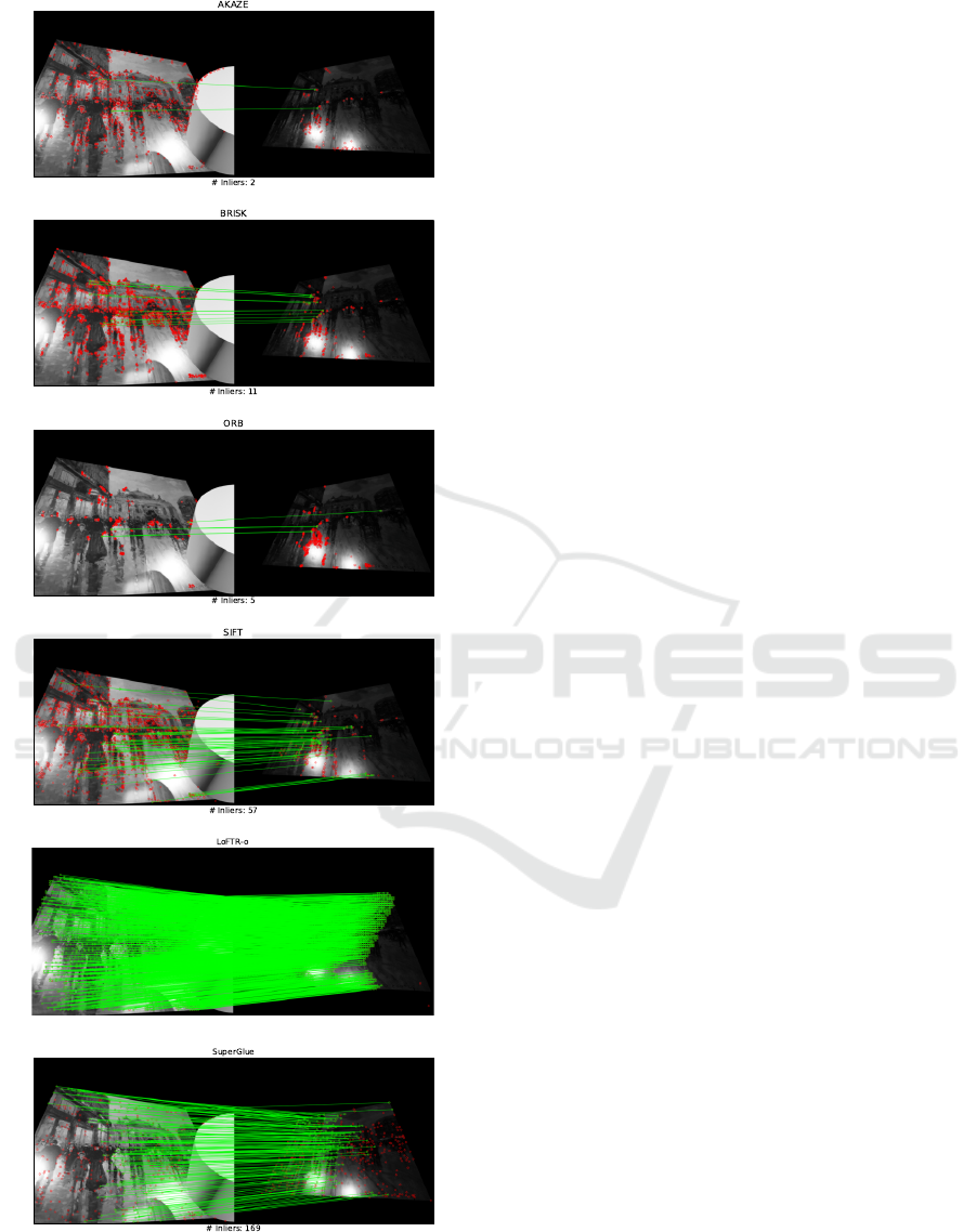
Figure 18: An overview of different keypoint detectors with

corresponding inliers.

Bradski, G. (2000). The OpenCV Library. Dr. Dobb’s Jour-

nal of Software Tools.

Butler, D. J., Wulff, J., Stanley, G. B., and Black, M. J.

(2012a). A naturalistic open source movie for optical

ﬂow evaluation. In A. Fitzgibbon et al. (Eds.), editor,

European Conf. on Computer Vision (ECCV), Part IV,

LNCS 7577, pages 611–625. Springer-Verlag.

Butler, D. J., Wulff, J., Stanley, G. B., and Black, M. J.

(2012b). A naturalistic open source movie for opti-

cal ﬂow evaluation. In Computer Vision–ECCV 2012:

12th European Conference on Computer Vision, Flo-

rence, Italy, October 7-13, 2012, Proceedings, Part VI

12, pages 611–625. Springer.

Cand

es, E. J., Li, X., Ma, Y., and Wright, J. (2011). Robust

principal component analysis? Journal of the ACM

(JACM), 58(3):1–37.

Cao, S.-Y., Hu, J., Sheng, Z., and Shen, H.-L. (2022). It-

erative deep homography estimation. In Proceedings

of the IEEE/CVF Conference on Computer Vision and

Pattern Recognition (CVPR), pages 1879–1888.

Chang, C.-H., Chou, C.-N., and Chang, E. Y. (2017).

Clkn: Cascaded lucas-kanade networks for image

alignment. In Proceedings of the IEEE conference on

computer vision and pattern recognition, pages 2213–

2221.

Chen, T., Kornblith, S., Norouzi, M., and Hinton, G. (2020).

A simple framework for contrastive learning of visual

representations.

DeTone, D., Malisiewicz, T., and Rabinovich, A. (2016).

Deep image homography estimation. arXiv preprint

arXiv:1606.03798.

DeTone, D., Malisiewicz, T., and Rabinovich, A. (2018).

Superpoint: Self-supervised interest point detection

and description. In Proceedings of the IEEE con-

ference on computer vision and pattern recognition

workshops, pages 224–236.

Dmytro Mishkin, Filip Radenovic, J. M. (2018). Re-

peatability Is Not Enough: Learning Discriminative

Afﬁne Regions via Discriminability. In Proceedings

of ECCV.

Erlik Nowruzi, F., Laganiere, R., and Japkowicz, N. (2017).

Homography estimation from image pairs with hier-

archical convolutional networks. In Proceedings of

the IEEE international conference on computer vision

workshops, pages 913–920.

Goyette, N., Jodoin, P.-M., Porikli, F., Konrad, J., and Ish-

war, P. (2012). Changedetection. net: A new change

detection benchmark dataset. In 2012 IEEE computer

society conference on computer vision and pattern

recognition workshops, pages 1–8. IEEE.

Hartley, R. and Zisserman, A. (2003). Multiple view geom-

etry in computer vision. Cambridge university press.

Jodoin, P.-M., Maddalena, L., Petrosino, A., and Wang, Y.

(2017). Extensive benchmark and survey of modeling

methods for scene background initialization. IEEE

Transactions on Image Processing, 26(11):5244–

5256.

Kalsotra, R. and Arora, S. (2019). A comprehensive survey

of video datasets for background subtraction. IEEE

Access, 7:59143–59171.

SIDAR: Synthetic Image Dataset for Alignment & Restoration

187

Kligler, N., Katz, S., and Tal, A. (2018). Document en-

hancement using visibility detection. In Proceedings

of the IEEE Conference on Computer Vision and Pat-

tern Recognition, pages 2374–2382.

Kluger, F., Brachmann, E., Ackermann, H., Rother, C.,

Yang, M. Y., and Rosenhahn, B. (2020). Consac: Ro-

bust multi-model ﬁtting by conditional sample con-

sensus. In Proceedings of the IEEE Conference on

Computer Vision and Pattern Recognition (CVPR).

Kwiatkowski, M. and Hellwich, O. (2022). Specularity,

shadow, and occlusion removal from image sequences

using deep residual sets. In VISIGRAPP (4: VISAPP),

pages 118–125.

Kwiatkowski, M., Matern, S., and Hellwich, O. (2022).

Diar: Deep image alignment and reconstruction using

swin transformers. In International Joint Conference

on Computer Vision, Imaging and Computer Graph-

ics, pages 248–267. Springer.

Le, H., Liu, F., Zhang, S., and Agarwala, A. (2020). Deep

homography estimation for dynamic scenes. In Pro-

ceedings of the IEEE/CVF Conference on Computer

Vision and Pattern Recognition (CVPR).

Li, Z. and Snavely, N. (2018). Megadepth: Learning single-

view depth prediction from internet photos. In Com-

puter Vision and Pattern Recognition (CVPR).

Lin, C.-H., Ma, W.-C., Torralba, A., and Lucey, S. (2021).

Barf: Bundle-adjusting neural radiance ﬁelds. In

IEEE International Conference on Computer Vision

(ICCV).

Lin, T.-Y., Maire, M., Belongie, S., Hays, J., Perona, P.,

Ramanan, D., Doll

ar, P., and Zitnick, C. L. (2014).

Microsoft coco: Common objects in context. In Com-

puter Vision–ECCV 2014: 13th European Confer-

ence, Zurich, Switzerland, September 6-12, 2014, Pro-

ceedings, Part V 13, pages 740–755. Springer.

Lindenberger, P., Sarlin, P.-E., Larsson, V., and Pollefeys,

M. (2021). Pixel-Perfect Structure-from-Motion with

Featuremetric Reﬁnement. In ICCV.

Lowe, D. G. (1999). Object recognition from local scale-

invariant features. In Proceedings of the seventh

IEEE international conference on computer vision,

volume 2, pages 1150–1157. Ieee.

Mandal, M. and Vipparthi, S. K. (2021). An empirical re-

view of deep learning frameworks for change detec-

tion: Model design, experimental frameworks, chal-

lenges and research needs. IEEE Transactions on In-

telligent Transportation Systems.

Mikolajczyk, K. and Schmid, C. (2005). A perfor-

mance evaluation of local descriptors. IEEE trans-

actions on pattern analysis and machine intelligence,

27(10):1615–1630.

Mishchuk, A., Mishkin, D., Radenovic, F., and Matas,

J. (2017). Working hard to know your neighbor's

margins: Local descriptor learning loss. In Guyon,

I., Luxburg, U. V., Bengio, S., Wallach, H., Fer-

gus, R., Vishwanathan, S., and Garnett, R., editors,

Advances in Neural Information Processing Systems,

volume 30. Curran Associates, Inc.

Qu, L., Tian, J., He, S., Tang, Y., and Lau, R. W. (2017). De-

shadownet: A multi-context embedding deep network

for shadow removal. In Proceedings of the IEEE Con-

ference on Computer Vision and Pattern Recognition,

pages 4067–4075.

Riba, E., Mishkin, D., Ponsa, D., Rublee, E., and Brad-

ski, G. (2020). Kornia: an open source differentiable

computer vision library for pytorch. In Proceedings of

the IEEE/CVF Winter Conference on Applications of

Computer Vision, pages 3674–3683.

Roberts, M., Ramapuram, J., Ranjan, A., Kumar, A.,

Bautista, M. A., Paczan, N., Webb, R., and Susskind,

J. M. (2021). Hypersim: A photorealistic synthetic

dataset for holistic indoor scene understanding. In

International Conference on Computer Vision (ICCV)

2021.

Rublee, E., Rabaud, V., Konolige, K., and Bradski, G.

(2011). Orb: An efﬁcient alternative to sift or surf.

In 2011 International conference on computer vision,

pages 2564–2571. Ieee.

Sarlin, P.-E., DeTone, D., Malisiewicz, T., and Rabinovich,

A. (2020). Superglue: Learning feature matching

with graph neural networks. In Proceedings of the

IEEE/CVF conference on computer vision and pattern

recognition, pages 4938–4947.

Schops, T., Schonberger, J. L., Galliani, S., Sattler, T.,

Schindler, K., Pollefeys, M., and Geiger, A. (2017).

A multi-view stereo benchmark with high-resolution

images and multi-camera videos. In Proceedings of

the IEEE Conference on Computer Vision and Pattern

Recognition, pages 3260–3269.

Shen, X., Darmon, F., Efros, A. A., and Aubry, M. (2020).

Ransac-ﬂow: generic two-stage image alignment. In

16th European Conference on Computer Vision.

Sun, J., Shen, Z., Wang, Y., Bao, H., and Zhou, X. (2021).

LoFTR: Detector-free local feature matching with

transformers. CVPR.

Tan, W. R., Chan, C. S., Aguirre, H., and Tanaka, K. (2019).

Improved artgan for conditional synthesis of natural

image and artwork. IEEE Transactions on Image Pro-

cessing, 28(1):394–409.

Tareen, S. A. K. and Saleem, Z. (2018). A comparative anal-

ysis of sift, surf, kaze, akaze, orb, and brisk. In 2018

International conference on computing, mathematics

and engineering technologies (iCoMET), pages 1–10.

IEEE.

Toyama, K., Krumm, J., Brumitt, B., and Meyers, B.

(1999). Wallﬂower: Principles and practice of back-

ground maintenance. In Proceedings of the seventh

IEEE international conference on computer vision,

volume 1, pages 255–261. IEEE.

Truong, P., Danelljan, M., and Timofte, R. (2020). GLU-

Net: Global-local universal network for dense ﬂow

and correspondences. In IEEE Conference on Com-

puter Vision and Pattern Recognition, CVPR 2020.

Truong, P., Danelljan, M., Timofte, R., and Gool, L. V.

(2021). Pdc-net+: Enhanced probabilistic dense cor-

respondence network. In Preprint.

Vacavant, A., Chateau, T., Wilhelm, A., and Lequievre,

L. (2013). A benchmark dataset for outdoor fore-

ground/background extraction. In Computer Vision-

ACCV 2012 Workshops: ACCV 2012 International

VISAPP 2024 - 19th International Conference on Computer Vision Theory and Applications

188

Workshops, Daejeon, Korea, November 5-6, 2012,

Revised Selected Papers, Part I 11, pages 291–300.

Springer.

Wang, J., Li, X., Hui, L., and Yang, J. (2017). Stacked

conditional generative adversarial networks for jointly

learning shadow detection and shadow removal.

Weiss, Y. (2001). Deriving intrinsic images from image se-

quences. In Proceedings Eighth IEEE International

Conference on Computer Vision. ICCV 2001, vol-

ume 2, pages 68–75. IEEE.

Wong, H. S., Chin, T.-J., Yu, J., and Suter, D. (2011).

Dynamic and hierarchical multi-structure geometric

model ﬁtting. In 2011 International Conference on

Computer Vision, pages 1044–1051. IEEE.

Zaheer, M., Kottur, S., Ravanbakhsh, S., Poczos, B.,

Salakhutdinov, R. R., and Smola, A. J. (2017). Deep

sets. Advances in neural information processing sys-

tems, 30.

SIDAR: Synthetic Image Dataset for Alignment & Restoration

189