Improvement of Ghost Imaging-OCT High-Resolution Real-Time

Imaging

Decai Huyan

and Tatsuo Shiina

Graduate School of Science and Engineering, Chiba University, Chiba-shi, Japan

Keywords:

OCT, Ghost Imaging, Machine Learning.

Abstract:

We previously proposed a novel system composed of GI (ghost imaging) and OCT (optical coherence tomog-

raphy) to solve the problem of scattering and absorption by OCT measuring within scattering media. It is

named GI-OCT. And we successfully obtained images of scattering media and target separately in a 2× 2mm.

In this paper, we improve a new computational approach to deal with the signiﬁcant computational demands

arising from increased image resolution. Using DIP (deep image prior) technique, we obtained images with

minimal measurement data compared to traditional computational methods. In the simulation, the number of

measurements required to obtain a clear image was reduced to 10%.

1 INTRODUCTION

Optical Coherence Tomography (OCT) is an ad-

vanced imaging technique capable of generating

high-resolution tomographic images through a non-

contact, non-invasive approach in non-homogeneous

mediums (Huang et al., 1991). Operating on the prin-

ciple of low-coherence interference, OCT combines

reﬂected light from measurement and reference paths

to reconstruct the optical property distribution of an

object in the depth direction. Widely employed in

commercial applications, OCT has demonstrated re-

markable success in ophthalmology, providing intri-

cate images of the inner retina. Recently, its applica-

tion has extended to cardiology and dermatology for

diagnostic purposes (Gambichler et al., 2005; Sinclair

et al., 2015; Schwartz et al., 2017; Spaide et al., 2018;

Vabre et al., 2012). Furthermore, OCT ﬁnds utility

in various biomedical scenarios, particularly in mul-

tilayer scattering media such as organs and skin (Kir-

illin et al., 2008). This imaging technique is crucial

in early skin cancer detection and other biomedical

applications.

In recent years, ghost imaging (GI) techniques

have attracted attention for their ability to separate

signals from noise. Since publishing ”ghost imag-

ing using a single detector (Bromberg et al., 2009)”,

GI has been used in many ﬁelds (Lindell and Wet-

https://orcid.org/0000-0002-2490-0439

https://orcid.org/0000-0001-9292-4523

zstein, 2020; Shapiro, 2008; Katkovnik and Astola,

2012; Ryczkowski et al., 2016; Devaux et al., 2016;

Zhao et al., 2012; Chen and Chen, 2013; Olivieri

et al., 2020; Miot et al., 2019). Researchers in this

paper demonstrated that a single probe can illuminate

a sample multiple times with different light patterns,

and reconstruct an image based on the relationship be-

tween the reﬂected light total intensity and the illumi-

nated light pattern.

We previously proposed a novel system consisting

of GI and OCT to solve the scattering and absorp-

tion challenges encountered in OCT measurements

in scattering media, named GI-OCT (Huyan et al.,

2022). This challenge refers to the fact that during

OCT measurements in scattering media, the target

signal is always affected by light attenuation and scat-

tering in the scattering media when the measured light

propagates in the depth direction. The scattering me-

dia may change the direction of the measured light,

causing a time delay. This makes it difﬁcult to ob-

tain the exact shape of the target and a proper image

of the target in the scattering media. GI-OCT uti-

lizes the ability of GI to reconstruct an image even

when the signal-to-noise ratio is low due to scatter-

ing. Using GI-OCT, obtaining an image of the target

without scattering effects is possible. We successfully

obtained no scattering effects images of the target in

a scattering media in the range of 2 × 2mm (Huyan

et al., 2023). In practical OCT applications, high res-

olution and quick calculation are required for precise

and accurate results. However, in GI-OCT, a large

Huyan, D. and Shiina, T.

Improvement of Ghost Imaging-OCT High-Resolution Real-Time Imaging.

DOI: 10.5220/0012391000003651

Paper published under CC license (CC BY-NC-ND 4.0)

In Proceedings of the 12th International Conference on Photonics, Optics and Laser Technology (PHOTOPTICS 2024), pages 28-35

ISBN: 978-989-758-686-6; ISSN: 2184-4364

number of single-pixel measurements are required be-

cause each sample contains only a small amount of

information about the object. Speciﬁcally, in the com-

putational method, the result that best obtains an im-

age of N pixels requires at least M = N measurements

to meet β = M/N = 100%, where β represents the

sampling rate. In our practical measurement situa-

tion, measurements of M > 4N are required to ob-

tain good-quality images. This leads to a positive cor-

relation between the number of pixels of the object

and the data acquisition time, which is almost impos-

sible to accomplish for instantaneous high-resolution

images. Therefore, an important and long-term goal

of advancing GI-OCT is to reduce the value β while

maintaining good resolution, thus reducing the bur-

den of data acquisition and obtaining better imaging

quality.

With the development of deep learning, more

and more methods are being used to solve GI com-

putations. For example, deep learning-based GI

(GIDL)(Lyu et al., 2017) and Deep Image Prior

(DIP)(Lempitsky et al., 2018). This GIDL technique

uses a deep neural network (DNN) to learn from a

large number of input-output data pairs in order to es-

tablish mapping relationships between them. How-

ever, the experiments require access to huge train-

ing sets, which is both time-consuming and laborious,

and the trained models can only reconstruct objects

similar to the training set well, and the generalization

challenge is the major problem.

DIP uses an untrained neural network as a con-

straint for image processing tasks such as denois-

ing, inpainting, and super-resolution. The genera-

tor network can be used without prior training, thus

eliminating the need for tens of thousands of la-

beled data. At the same time, this technique is used

for GI computation, Deep neural network Constraint

(GIDC) (Wang et al., 2022), which inputs the differ-

ential ghost imaging (DGI) reconstruction results into

a randomly initialized neural network (untrained) to

reconstruct remarkably high signal-to-noise ratio GI

images at very low sampling rates β.

Inspired by the GIDC concept, we install here the

DIP technique for GI-OCT, where the GI-OCT re-

construction results are input into a randomly initial-

ized neural network, and the results are computed by

the DIP technique to obtain good images at a small

number of measurements. This enables the GI-OCT

technique to obtain high resolution while reducing

the number of measurements accomplishing fast and

high-resolution measurements of biological samples.

In this paper, we have accomplished the applica-

tion of the DIP technique in a simulation to conﬁrm

the results for 64 × 64 at β = 10%, obtaining a clear

image. The calculation of 64 × 64 at β = 10% and

25% was accomplished in experiments, and a better

target image was obtained.

2 METHOD

2.1 Concept of GI-OCT

GI-OCT is the solution to the problem of scattering

media. The target in the scattering media (scatter-

ing sample) is simpliﬁed into two parts in OCT mea-

surements. The former part is the scatter layer be-

fore the light hits the target. The latter part is the tar-

get layer. By changing the reference path (A-scan)

and moving the probe orthogonally (B-scan), conven-

tional OCT can construct a 3-dimensional image of

the target layer in the scattering sample, as shown in

Figure 1. However, the measured intensity distribu-

tion from the target layer has been affected because

the image always has some uneliminated effects from

the former scattering layers. When OCT measures the

optical properties (transmittance and absorbance) of

the target layer, the former scattering layers’ distri-

bution may change the light direction, or delay the

received signal of the target layer due to the scatter’s

inﬂuence. As a result, the optical properties with the

scattering effect of the target layer are detected.

Target image

with scattering

Low coherence

light source

Reference

mirror

Scatter

Target

Scattering sample

light

probe

Photodiode

Data

process

Intensity

Time

Scatter signal

Figure 1: Setup of a conventional OCT, that produces the

target image with scattering inﬂuence.

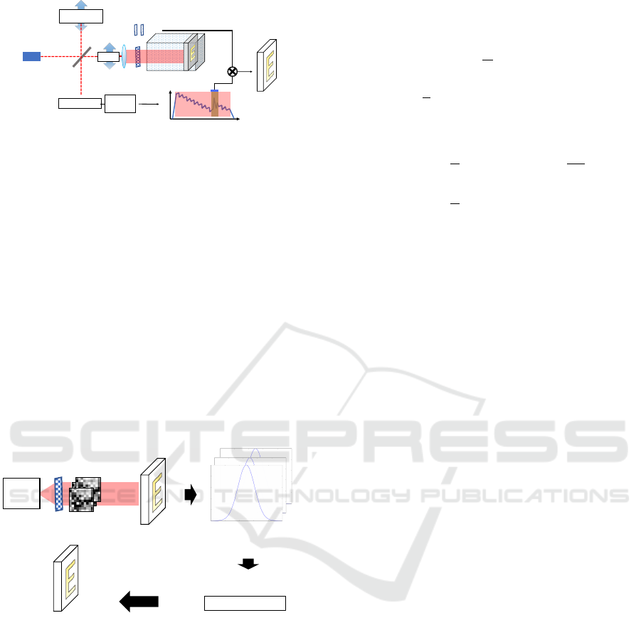
The GI-OCT concept is shown in Figure 2, where

light passes through an expander and a spatial light

modulator (SLM), and light patterns are generated to

illuminate the target layer within the scattering sam-

ple. A single detector collects light intensity from the

target and scatter layers. Each illuminated light pat-

tern in GI-OCT produces an A-scan signal, which is a

series of light intensities in the depth direction. With

the OCT axial resolution, these series of light intensi-

ties can be separated as the summed intensity of each

layer distribution. With the GI method, the correlation

between the different light patterns and the summed

intensity of each separated layer is calculated after re-

peated measurements using different light patterns.

Improvement of Ghost Imaging-OCT High-Resolution Real-Time Imaging

Low coherence

light source

Reference

mirror

Photodiode

Data

process

Intensity

Time

Scatter signal

SLM

····

probe

Target image

without scattering

Figure 2: Setup of GI-OCT, that produces the scatter image

that can be used to generate the target image without the

scattering inﬂuence.

Instead of conventional OCT setups using a point

measurement, GI-OCT uses a 2D measurement. This

detector can simultaneously measure lights going in

other directions or the signal delayed by scattering

media. The results show them as scatter distributions.

After this, we can compute the distribution of the tar-

get layer using the GI method and the distribution of

the former scattering layer using the same method.

The former scatter layer distribution can be used to

correct the optical properties of the target layer.

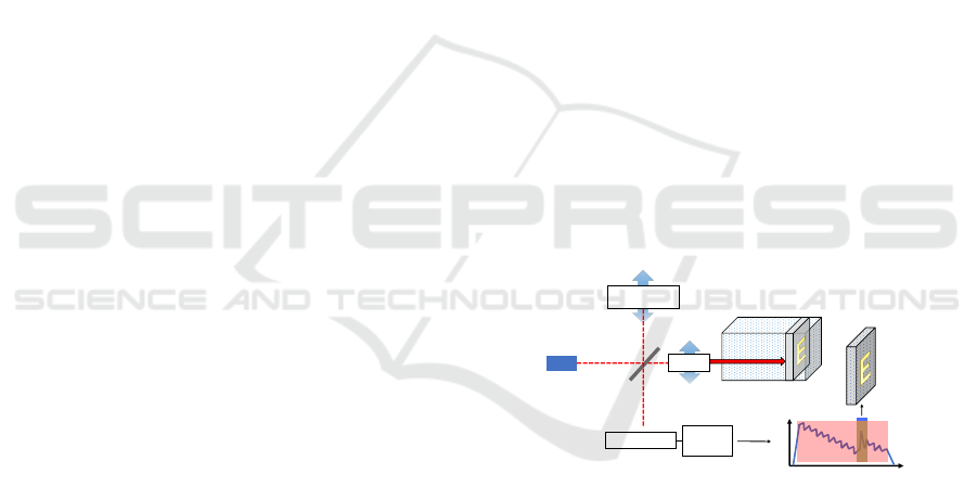
2.2 The Calculation of GI-OCT

Figure 3 shows the schematic diagram of the GI-OCT

method for detecting the distribution of sample layers.

Time

Intensity

Intensity of OCT signal

Pattern

Result of GI-OCT

probe

Sample layer

Calculation of GI

DMD

Figure 3: Setup of GI-OCT, that produces the scatter image

that can be used to generate the target image without the

scattering inﬂuence.

In order to obtain the OCT light intensity, different

patterns of light from the digital micromirror device

(DMD) chip illuminate the sample layer, as deﬁned

in Eq. (1),

= α

β(sample) (1)

where α

is the light pattern with m × m speckles

illuminated from the DMD chip; β(sample) is the

transmittance distribution of the sample layer; I

the received light intensity summed from all speck-

les’ intensities, which is the OCT interference light

intensity. β

′

(sample) is the reconstructed image of

the sample layer’s transmittance distribution using the

computational ghost imaging (CGI) method by calcu-

lating the correlation between α

and I

′

(sample)

CGI

∑

n=1

(α

− ⟨α

⟩)I

(2)

where ⟨α

⟩ =

∑

n=1

is the average of light pat-

terns.

The DGI is calculated using Eq. (3),

′

(sample)

DGI

∑

n=1

(α

− ⟨α

⟩)(I

−

⟨I⟩

⟨I

′

⟩

′

)

∑

n=1

(α

− ⟨α

⟩)I

⋆

(3)

where I

′

is the total light intensity of each light pattern

without sample, and I

⋆

is called the light transmission

relative variance. Depending on the light transmission

relative variance, DGI can have signal-to-noise ratios

several orders of magnitude higher than CGI.

2.3 Faster Calculation

Because DGI requires a large amount of data, we use

the GIDC technique in order to increase the computa-

tional speed and reduce the measurement time. GIDC

provides the resulting DGI reconstruction into a ran-

domly initialized neural network (untrained). After

that, the output of the neural network is used as esti-

mated values of the high-quality GI image. Finally,

the weights of the neural network are updated to min-

imize the error between the measured and estimated

values. As the error is minimized, the output of the

neural network converges to a high-quality image.

For the proposed GIDC, the function for reconstruct-

ing the object image is as Eq.(4) and (5).

⋆

= argmin

θ∈Θ

∥ f

(z) − β

′

(sample)

DGI

∥

(4)

′

(sample)

GIDC

= f

⋆

(z) (5)

Where f is the neural network, Θ is the network

parameter (obtained by random initialization at the

beginning), z is a ﬁxed random code initially inputted

into the network, θ

⋆

is the optimal solution of the pa-

rameter obtained by training, and β

′

(sample)

GIDC

the optimal output of the network, which is the re-

constructed high-quality image. argmin

θ∈Θ

is the ar-

gument of the minimum, which makes the value of

the variable when the formula obtains the minimum

value.

Figure 4 shows the results obtained from the ex-

periment using the original data from GIDC (data

from GIDC)(Wang et al., 2022). Figure 4 shows the

results of GIDC iterations on DGI reconstructed im-

ages. Figure 4 (a) shows the DGI results, in 64 × 64

PHOTOPTICS 2024 - 12th International Conference on Photonics, Optics and Laser Technology

size, computed 400 times. Figure 4 (b) results from

training 0 times using the neural network. Figure 4

times.

(a) (b)

Figure 4: The results of (a) is DGI uses 64 × 64 to compute

400 times. (b), (c) and (d) are the results of training 0, 100

and 200 times.

3 SIMULATION

This simulation utilizes the GIDC network structure

derived from the U-network. Algorithm 1 describes

the main progress. The weights in the neural network

are updated using an Adam optimizer with a learning

rate α = 0.05. The leakage parameter of Leaky ReLU

is 0.2. The regularization parameter of TV is 10

−10

L refers to the number of iterations.

Data: DGI’s result, α = 0.05, Leaky

ReLU=0.2, TV=10

−10

, L=400

Result: GI reconstruction with GIDC

initialization: a randomly initialized

parameters Θ in neural network (untrained).;

while Step=1,2,3. . . L do

(z) = θ ∈ Θ;

= MSE( f

(z) − β

′

(sample)

DGI

);

θ = ADAM(L

,α)

end

Algorithm 1: The algorithms of GIDC.

The sample used for the simulation is the character

’E’, as shown in Figure 5.

Firstly, the corresponding light intensity ( I) was

obtained after illuminating the sample (β) with 64 ×

64 size random pattern (α). Then, using the DGI cal-

culation method of Eq. (3), the calculated result of

the sample (β

′

) was obtained by employing the pat-

tern (α) and the light intensity ( I). Finally, the calcu-

lated results were applied to the GIDC to obtain the

results for 0, 100, and 200 iterations.

Figure 6 (a) shows the DGI results for character

’E’ at 400 calculations with size 64 × 64. Figure 6

(b) shows the result of 0 times training using neural

network. Figure 6 (c) and (d) show the results for

100 and 200 iterations. We succeeded in getting clear

images from only recognizable DGI images.

Figure 5: The character ’E’ is utilized in the simulation.

(a) (b)

Figure 6: The results of (a) is DGI uses 64 × 64 to compute

400 times. (b), (c) and (d) are the results of training 0, 100

and 200 times.

Improvement of Ghost Imaging-OCT High-Resolution Real-Time Imaging

4 EXPERIMENT AND SETUP

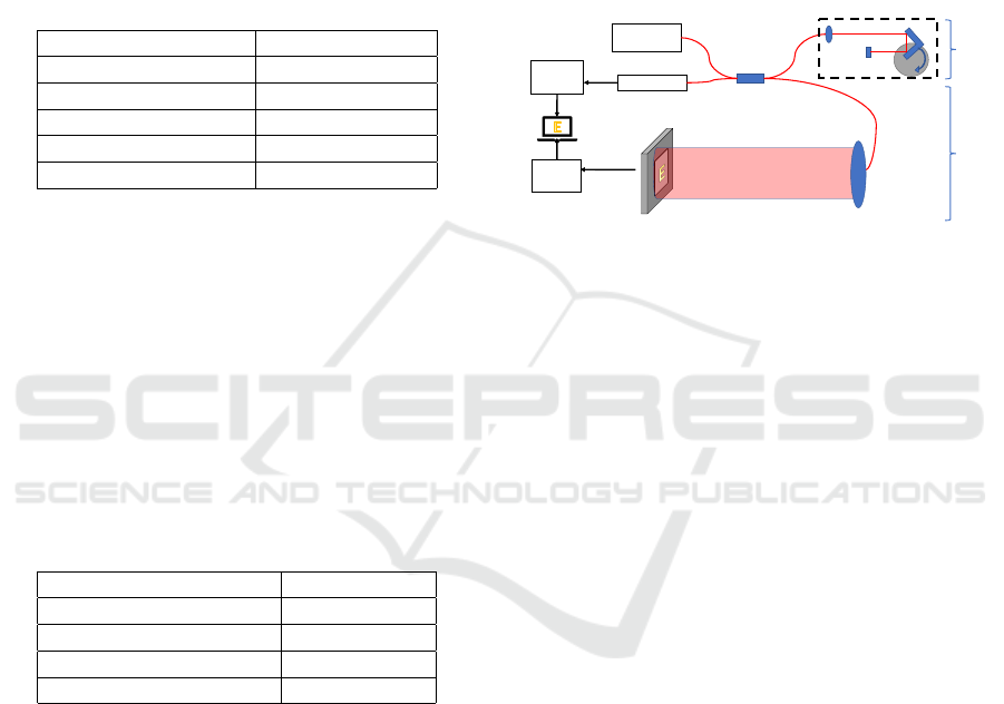
Figure 7 illustrates the experimental setup for GI-

OCT.

In the GI-OCT, the axial resolution is equivalent to

coherence length, deﬁned as δz = 0.44λ

/∆λ, where

= 856 nm is the central wavelength of a high-

power Superluminescent diodes (SLD) light source

with Gaussian distribution, and the equipment spec-

iﬁcations are shown in Table 1.

Table 1: SLD speciﬁcation of GI-OCT.

Manufacturer THORLABS

Model number SLD850S-A20W

Center wavelength 860 nm

Spectral band width 28 nm

Coherence length 11.6µm

Optical power[MAX] 30 mW

To make illumination patterns, the GI-OCT beam

must spread and reﬂect part of the light. In this study,

a high-power SLD was prepared in order to validate

the new GI-OCT algorithm. The reference path length

scanning mechanism is composed of a steady rotat-

ing motor and a ﬁxed mirror that completes the axial

scanning process(Shiina et al., 2003). The measure-

ment path is equipped with an optical probe, and a

varifocal collimator makes a beam of 2 mm diameter.

Meanwhile, the high-speed DMD chip is set in the

measurement path, and its speciﬁcations are shown in

Table 2.

Table 2: DMD speciﬁcation of GI-OCT.

Manufacturer TI

Model number DLP2010LC

Illumination wavelength 860 nm (90%)

Array diagonal 5.29 mm

Output frame rate 240 Hz

On the DMD chip, micromirrors are arranged in

a matrix of 854 × 480, with a total size of 4.61 ×

2.59mm. Each micromirror has a size of 5.4 × 5.4 µm

and a deﬂection angle of ±17 degrees on the diagonal

axis, divided into two states, ”on” and ”off”. In or-

der to reﬂect pattern light back to the collimator, the

DMD chip is tilted +17 degrees along the diagonal.

The DMD chip was controlled to display a speckle

pattern within a 1.5 × 1 mm

DMD chip area, 64 ×

64 were applied in this experiment.

The character ”E” also shown on the DMD, which

overlaps the illumination pattern, was used as the tar-

get object for this experiment to be able to focus on

the reconstruction effect, as shown in Figure 5. In ad-

dition, the DMD chip was placed in the interference

region of the OCT so that the OCT measurements are

efﬁcient in terms of light reﬂection and stable in terms

of light intensity, which makes it easy to reconstruct

the results from the images.

In this paper, different number of measurements

were prepared: 410 and 1000 measurements. In ac-

tual measurements, there will be a lot of noise and

bias affecting the experimental results. It is not pos-

sible to get the β=10% in the simulation results and

the number of measurements needs to be increased to

enhance the results.

High power

SLD 856nm

Photodiode

Reference path

OCT

Pattern

Intensity

DMD

Collimator

𝜶

𝒏

𝑰

𝒏

Image

Reconstruction

Figure 7: Experiment setup of GI-OCT.

5 RESULT

We have used the character ’E’ of Figure 5 as the

target image. Figure 8 shows the results at different

numbers of iterations with the GIDC method and the

DGI results, with the reconstructed image of the GI-

OCT device at the actual number of measurements of

410, with a measurement pattern size of 64× 64. Fig-

ure 8 (a) shows the results of the DGI method. In this

result, little information is obtained for each pattern, a

large number of measurements are required to obtain

a recognizable target image, and the reconstructed im-

age has the shape of the target image. Figures 8(b),

(c), (d), and (e) show the results for 0, 100, 200, 300,

and 400 iterations. Among these results, the 0th result

is the worst, which is consistent with the simulation

result (Fig.6 (a)). However, from the 100th iteration,

the iteration results hardly change anymore and the

reconstructed image is hardly visible as the target im-

age.

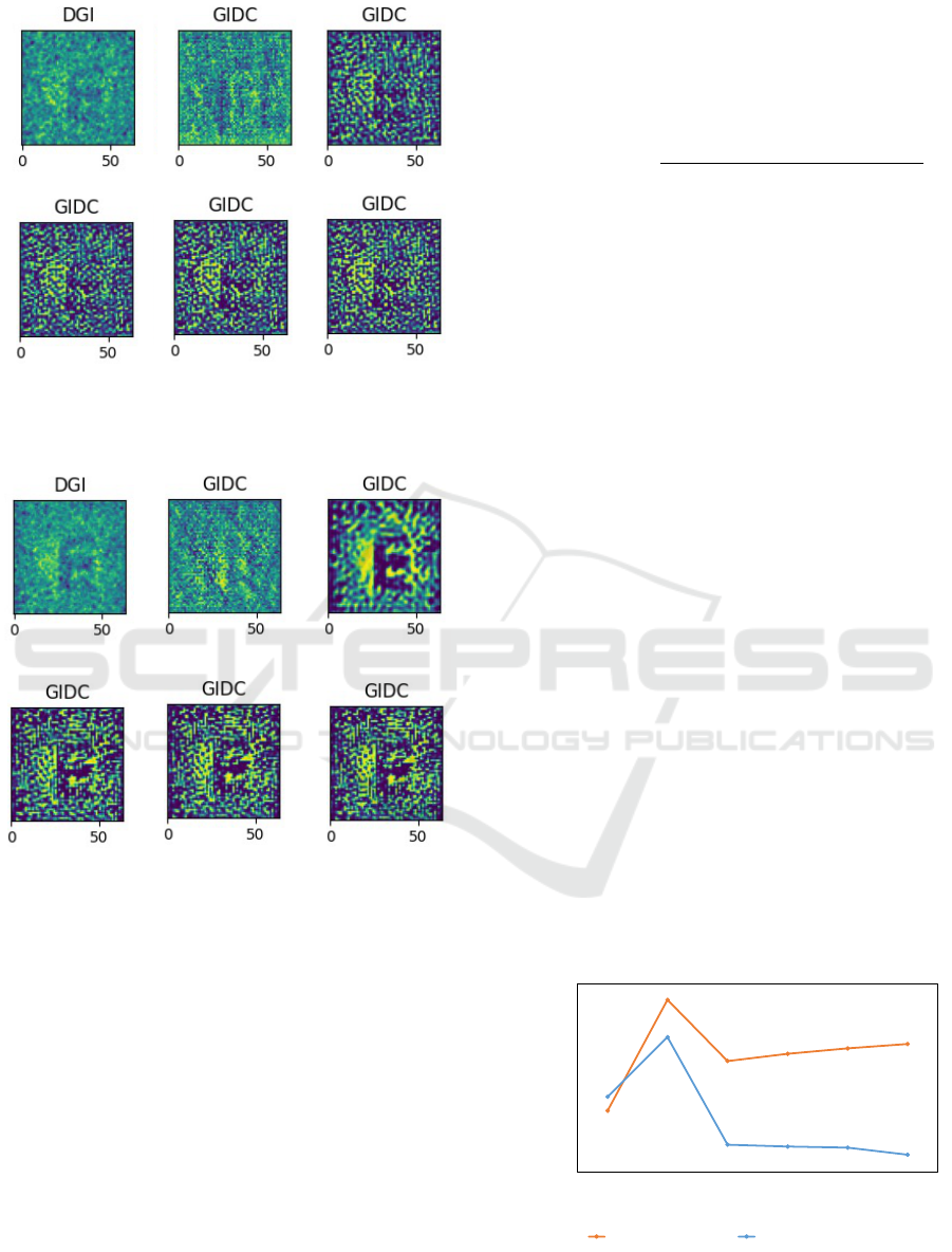
Figure 9 shows the results using the GIDC method

at different numbers of iterations and the DGI results

with the reconstructed image of the GI-OCT device

at the actual number of measurements of 1000, with

a measurement pattern size of 64 × 64. Figure 9 (a)

shows the results of the DGI method. This result is

almost identical to the DGI result in Figure 8 (a). Fig-

ures 9 (b), (c), (d), and (e) show the 0th, 100th, 200th,

300th, and 400th iteration results. Among these re-

sults, the same 0th result is the worst. The character

PHOTOPTICS 2024 - 12th International Conference on Photonics, Optics and Laser Technology

(a) (b) 0

(d) 200 (e) 300 (f) 400

Figure 8: The results of each iteration by GIDC method and

DGI method in 410 measurements.

(a) (b) 0

(d) 200 (e) 300 (f) 400

Figure 9: The results of each iteration by GIDC method and

DGI method in 1000 measurements.

”E” is clearly visible in the 100th result image. After

200 times iterations, the iteration results progressively

worsen, probably due to overﬁtting.

6 DISCUSSION

In this paper, the structural similarity index method

(SSIM) is introduced for the purpose of evaluating

the reconstructed images. SSIM is a method for pre-

dicting the perceived quality of two images. SSIM is

close to 1, indicating that the perceived structure of

the two images is consistent, while SSIM is close to

0, indicating that the images are unrelated. The SSIM

results are used to make a subjective judgment of the

clarity of the image character ”E”, a positive SSIM

value means that the reconstructed image is positively

correlated and a negative value means that it is nega-

tively correlated. The SSIM is used to evaluate the

quality of the reconstructed image.

SSIM(x,y) =

(2µ

+(K

)(2σ

+(K

)

(µ

+µ

+(K

)(σ

+σ

+(K

)

(6)

here, x and y indicate the expected result and

the comparison result. µ is he mean value, σ is the

standard deviation, σ

is the covariance of x and y,

K1 = 0.01,K2 = 0.03, and L represents the maximum

possible pixel value in the image. The experimental

images are compressed between 0 and 1; here, L = 1.

We compared the SSIM results for different num-

ber of measurements with different number of itera-

tions.

By calculating the results of DGI and GIDC with

the SSIM values of Figure 5, we obtain Figure 10.

The SSIM of the DGI results for 410 measurements

is 0.003. The SSIM of the GIDC with each 100 itera-

tions, as shown by the blue line in Figure 10, reaches

a maximum of 0.004 at 100 iterations, and the re-

sults are negative after 200 iterations. The SSIM of

the DGI result for 1000 measurements was 0.005.

The SSIM of the GIDC with every 100 iterations, as

shown by the orange line in Figure 10, again reached

a maximum of 0.006 at 100 iterations, after which

they were all lower than 0.005 and did not change

much. The above two experiments proved that us-

ing the GIDC method enhanced the image results at

100 iterations. The experimentally obtained SSIM

has a very low value because the beam used in the

actual measurement of GI-OCT has a Gaussian distri-

bution. This resulted in a large difference between the

GI-OCT image and the character ’E’. There is a lot

of random noise, and it is impossible to achieve the

good results obtained in the simulation using β=10%.

A higher number of measurements is needed.

-0.006

-0.004

-0.002

0.002

0.004

0.006

0.008

0 100 200 300 400 500

SSIM

Iterations

1000 measurements 410 measurements

Figure 10: SSIM values of the GIDC results for different

numbers of iterations for 410 and 1000 measurements.

Improvement of Ghost Imaging-OCT High-Resolution Real-Time Imaging

7 CONCLUSION

In this study, we propose a new method applied to

GI-OCT to reduce the number of measurements. We

used the GIDC method, where the reconstruction re-

sults are added to a neural network, utilizing the fact

that neural networks are inherently low resistance to

natural signals and high resistance to noise.

We accomplished the reconstruction of GI-OCT

images in simulation and obtained clear images at

β=10%, greatly reducing the number of measure-

ments required for reconstruction in a size of 64 ×64.

It was experimentally veriﬁed that the method can en-

hance the reconstructed image at 100 iterations.

However, due to some problems, the SSIM values

could be better. This result is due to the background

light problem, which needs to be solved ﬁrst in the fu-

ture to get more correct results. It may also be due to

the fact that different GI calculation methods can af-

fect the imaging results. Therefore, it is necessary to

compare the effects of different GI calculation meth-

ods on the reconstructed images, which are computed

ghost imaging (CGI), pseudo-inverse ghost imaging

(PGI), and differential pseudo-inverse ghost imaging

(DPGI) (Don, 2019; Ferri et al., 2010; Zhang et al.,

2014). In addition, the number of speckles in the GI-

OCT illumination pattern can also greatly impact the

results and is an issue we need to research in the fu-

ture.

In the next step, we are going to apply this new

technique to obtain real-time, high-resolution images

of multilayers in scattering media of GI-OCT mea-

surements.

REFERENCES

Bromberg, Y., Katz, O., and Silberberg, Y. (2009). Ghost

imaging with a single detector. Physical Review A -

Atomic, Molecular, and Optical Physics, 79(5):1–4.

Chen, W. and Chen, X. (2013). Ghost imaging for three-

dimensional optical security. Applied Physics Letters,

103(22):1–5.

Devaux, F., Moreau, P.-A., Denis, S., and Lantz, E.

(2016). Computational temporal ghost imaging. Op-

tica, 3(7):698.

Don, M. (2019). An Introduction to Computational Ghost

Imaging with Example Code.

Ferri, F., Magatti, D., Lugiato, L. A., and Gatti, A. (2010).

Differential ghost imaging. Physical Review Letters,

104(25):1–4.

Gambichler, T., Moussa, G., Sand, M., Sand, D., Altmeyer,

P., and Hoffmann, K. (2005). Applications of opti-

cal coherence tomography in dermatology. Journal of

Dermatological Science, 40(2):85–94.

Huang, D., Swanson, E. A., Lin, C. P., Schuman, J. S., Stin-

son, W. G., Chang, W., Hee, M. R., Flotte, T., Gregory,

K., Puliaﬁto, C. A., and Fujimoto, J. G. (1991). Opti-

cal coherence tomography. Science, 254(5035):1178–

1181.

Huyan, D., Lagrosas, N., and Shiina, T. (2022). Target

imaging in scattering media using ghost imaging opti-

cal coherence tomography. APL Photonics, 7(8).

Huyan, D., Lagrosas, N., and Shiina, T. (2023). Optical

properties analysis of scattering media based on gi-oct

imaging. Photonics, 10(2).

Katkovnik, V. and Astola, J. (2012). Compressive sensing

computational ghost imaging. Journal of the Optical

Society of America A, 29(8):1556.

Kirillin, M. Y., Priezzhev, A. V., and Myllyl

a, R. (2008).

Role of multiple scattering in formation of OCT skin

images. Quantum Electronics, 38(6):570–575.

Lempitsky, V., Vedaldi, A., and Ulyanov, D. (2018). Deep

Image Prior. 2018 IEEE/CVF Conference on Com-

puter Vision and Pattern Recognition, 128(7):9446–

9454.

Lindell, D. B. and Wetzstein, G. (2020). Three-dimensional

imaging through scattering media based on confo-

cal diffuse tomography. Nature Communications,

11(1):1–8.

Lyu, M., Wang, W., Wang, H., Wang, H., Li, G., Chen,

N., and Situ, G. (2017). Deep-learning-based ghost

imaging. Scientiﬁc Reports, 7(1):1–6.

Miot, C. A. G. A., Yczkowski, P. I. R., Riberg, A. R. I. T. F.,

Udley, J. O. H. N. M. D., and Enty, G. O. G. (2019).

Ghost optical coherence tomography. 27(17):24114–

24122.

Olivieri, L., Gongora, J. S. T., Peters, L., Cecconi, V.,

Cutrona, A., Tunesi, J., Tucker, R., Pasquazi, A.,

and Peccianti, M. (2020). Hyperspectral terahertz

microscopy via nonlinear ghost imaging. Optica,

7(2):186.

Ryczkowski, P., Barbier, M., Friberg, A. T., Dudley, J. M.,

and Genty, G. (2016). Ghost imaging in the time do-

main. Nature Photonics, 10(3):167–170.

Schwartz, M., Levine, A., and Markowitz, O. (2017). Op-

tical coherence tomography in dermatology. Cutis,

100(3):163–166.

Shapiro, J. H. (2008). Computational ghost imaging.

Physical Review A - Atomic, Molecular, and Optical

Physics, 78(6):1–4.

Shiina, T., Moritani, Y., Ito, M., and Okamura, Y. (2003).

Long-optical-path scanning mechanism for optical co-

herence tomography. Applied Optics, 42(19):3795.

Sinclair, H., Bourantas, C., Bagnall, A., Mintz, G. S., and

Kunadian, V. (2015). OCT for the identiﬁcation of

vulnerable plaque in acute coronary syndrome. JACC:

Cardiovascular Imaging, 8(2):198–209.

Spaide, R. F., Fujimoto, J. G., Waheed, N. K., Sadda, S. R.,

and Staurenghi, G. (2018). Optical coherence tomog-

raphy angiography. Progress in Retinal and Eye Re-

search, 64(June 2017):1–55.

Vabre, L., Dubois, A., Boccara, C., Vabre, L., Dubois, A.,

Boccara, C., Vabre, L., Dubois, A., and Boccara, A. C.

PHOTOPTICS 2024 - 12th International Conference on Photonics, Optics and Laser Technology

(2012). Thermal-light full-ﬁeld optical coherence to-

mography.

Wang, F., Wang, C., Chen, M., Gong, W., Zhang, Y., Han,

S., and Situ, G. (2022). Far-ﬁeld super-resolution

ghost imaging with a deep neural network constraint.

Light: Science and Applications, 11(1):1–11.

Zhang, C., Guo, S., Cao, J., Guan, J., and Gao, F. (2014).

Object reconstitution using pseudo-inverse for ghost

imaging. Optics Express, 22(24):30063.

Zhao, C., Gong, W., Chen, M., Li, E., Wang, H., Xu, W.,

and Han, S. (2012). Ghost imaging lidar via sparsity

constraints. Applied Physics Letters, 101(14):1–4.

Improvement of Ghost Imaging-OCT High-Resolution Real-Time Imaging