Inferring Interpretable Semantic Cognitive Maps from

Noisy Document Corpora

Yahya Emara

, Tristan Weger

, Ryan Rubadue

, Rishabh Choudhary

, Simona Doboli

and Ali A. Minai

University of Cincinnati, Cincinnati, OH 45221, U.S.A.

Hosftra University, Hempstead, NY, 11549, U.S.A.

Keywords:

Semantic Spaces, Cognitive Maps, Semantic Clustering, Language Models, Interpretable Vector-Space

Embeddings.

Abstract:

With the emergence of deep learning-based semantic embedding models, it has become possible to extract

large-scale semantic spaces from text corpora. Semantic elements such as words, sentences and documents

can be represented as embedding vectors in these spaces, allowing their use in many applications. However,

these semantic spaces are very high-dimensional and the embedding vectors are hard to interpret for humans.

In this paper, we demonstrate a method for obtaining more meaningful, lower-dimensional semantic spaces,

or cognitive maps, through the semantic clustering of the high-dimensional embedding vectors obtained from

a real-world corpus. A key limitation in this is the presence of semantic noise in real-world document corpora.

We show that pre-ﬁltering the documents for semantic relevance can alleviate this problem, and lead to highly

interpretable cognitive maps.

1 INTRODUCTION

One of the most important recent advances in natu-

ral language processing is the development of high-

quality methods for embedding semantic entities such

as words (Mikolov et al., 2013; Pennington et al.,

2014), sentences (Conneau et al., 2017; Cer et al.,

2018; Reimers and Gurevych, 2019), and even en-

tire documents (Beltagy et al., 2020; Le and Mikolov,

2014) in semantic vector spaces. This is the key step

enabling applications such as document classiﬁcation

(Devlin et al., 2019), text summarization (Pang et al.,

2022), text segmentation (Lo et al., 2021), and – most

notably – generative language models such as Chat-

GPT (OpenAI, 2023a) and GPT-4 (OpenAI, 2023b).

However, almost all the embedding methods use large

(and deep) neural networks, resulting in semantic

spaces that are extremely high-dimensional and ab-

stract in the sense that the individual dimensions have

no semantic interpretation. We have recently devel-

oped an approach to building interpretable semantic

cognitive maps from domain-speciﬁc text corpora us-

ing document embedding and clustering, but that ap-

proach has been validated only on small, noise-free

corpora with very short documents (Choudhary et al.,

2021; Choudhary et al., 2022; Fisher et al., 2022). In

this paper, we show that semantic cognitive maps can

also be inferred from large corpora of longer, more

noisy documents by using sentence-level embedding

and relevance ﬁltering.

2 MOTIVATION

Cognitive maps (Tolman, 1948) are mental frame-

works that allow a set of entities, e.g., locations,

concepts, etc., to be represented such that the rela-

tionships between the entities are captured. While

the semantic spaces constructed by language mod-

els such as BERT (Devlin et al., 2019), Universal

Sentence Encoder (USE) (Cer et al., 2018), MPNet

(Song et al., 2020), and XLM (Lample and Conneau,

2019) provide powerful representational frameworks,

they cannot be considered human-interpretable cog-

nitive maps because of their high dimensionality and

abstractness. Also, these models are typically pre-

trained on very large, generic datasets, and are thus

not always suitable for domain-speciﬁc representa-

tions (though some can be ﬁne-tuned for this pur-

pose).

The immediate motivation for the research re-

742

Emara, Y., Weger, T., Rubadue, R., Choudhary, R., Doboli, S. and Minai, A.

Inferring Interpretable Semantic Cognitive Maps from Noisy Document Corpora.

DOI: 10.5220/0012389100003636

Paper published under CC license (CC BY-NC-ND 4.0)

In Proceedings of the 16th International Conference on Agents and Artiﬁcial Intelligence (ICAART 2024) - Volume 3, pages 742-749

ISBN: 978-989-758-680-4; ISSN: 2184-433X

ported in this paper is the application of tracking ideas

expressed during brainstorming sessions (Coursey

et al., 2019) in real-time, and using this to track the

generated ideas in real time. This requires a seman-

tic space in which the expressed ideas can be repre-

sented in terms that the human participants can un-

derstand and that is appropriate for the domain of the

brainstorming session, i.e., a semantic cognitive map.

One way to build such a cognitive map is to infer it

from a sufﬁciently large reference corpus of domain-

speciﬁc documents. A broader motivation for our re-

search comes from the rapid growth in the use of large

language models (LLMs) (OpenAI, 2023a; OpenAI,

2023b), which work by creating a series of embedding

vectors for text and image inputs that can then be used

for inference. Analyzing the semantics of these ab-

stract embedding vectors is an essential part of inter-

preting the internal functionality of trained LLM net-

works, and the clustering-based approach presented

in this paper is a step in that direction.

We have recently proposed an approach for build-

ing cognitive maps from reference corpora (Choud-

hary et al., 2021; Choudhary et al., 2022). In this

approach, the reference documents are embedded us-

ing a model such as MPNet or USE, compressed to a

somewhat lower dimensionality using principal com-

ponents analysis retaining 95% variance (PCA95),

and then clustered adaptively to identify distinct re-

gions in the (still quite high-dimensional and ab-

stract) PCA95 space where reference document data

is dense, indicating that these regions are meaningful

for the domain. The clusters of reference data are each

characterized in terms of their keywords to provide in-

terpretability, and the centroids of these clusters are

used as the meaningful landmarks of the cognitive

map. We have shown that the approach works well if

the reference corpus consists of short, semantically-

focused, domain-speciﬁc, noise-free documents such

as descriptions of speciﬁc items in a domain-speciﬁc

list. However, such corpora are not easily available

for most domains. The work reported in the present

paper adapts the approach to work with large refer-

ence corpora comprising long, real-world documents.

This raises two problems: 1) In contrast to small doc-

uments, each long document contains a multiplicity

of topics, so embedding whole documents will not

produce meaningful clusters; and 2) Long documents

often include text that is not relevant to the domain

but is present only for stylistic reasons, thus adding

semantic noise to the documents. We address prob-

lem 1 by decomposing documents into individual sen-

tences and treating each sentence as a semantic ele-

ment for clustering, while problem 2 is addressed by

ﬁltering out sentences deemed irrelevant to the corpus

as whole. The results show that this approach works

well on substantial real-world corpora, one of which

is used as the reference corpus for this paper.

An important aim of the method we report is that it

should be systematic, i.e., it produces cognitive maps

with a quantitative quality metric, and allows a prin-

cipled selection of dimensionality. We achieve this by

deﬁning a cluster semantic coherence metric and us-

ing it to select the optimal number of clusters and to

evaluate the ﬁnal set obtained. We also use the clus-

tering process to remove additional semantic noise

from the dataset, which could be useful for other ap-

plications.

3 METHODS

3.1 Source Dataset

While we have evaluated our method on several

datasets, the results in this study are based on the

United States Presidential Speeches dataset avail-

able on Kaggle (Lilleberg, 2020), which contains a

comprehensive collection of speeches delivered by

all the U.S. presidents from Washington to Trump.

Our analysis focused speciﬁcally on the period from

Ronald Reagan to Donald Trump, encompassing 229

speeches and 45,639 sentences. Thus, each speech

consists of 200 sentences on average, which is a sig-

niﬁcant document length. Also, the speeches are all

from the domain of governance and politics, so the

corpus is domain-speciﬁc, albeit from a rather diverse

domain.

3.2 Overview

The process followed in the construction and evalu-

ation of the cognitive maps comprises the following

steps:

Sentence Embedding: All the documents in the

reference corpus are separated into individual sen-

tences, giving the sentence corpus (SC). Each sen-

tence in the SC is embedded into a semantic vector

space using a sentence embedding model. Based on

our previous work that considered and compared sev-

eral models for this (Choudhary et al., 2021; Choud-

hary et al., 2022), we use the MPNet model (Song

et al., 2020) for the embedding without any ﬁne tun-

ing. This produces a 768-dimensional vector for each

sentence in the SC. The set of all sentence vectors in

the SC is termed the unﬁltered sentence set (USS).

Short Sentence Removal: The number of tokens

in each sentence are counted. All sentences with three

or fewer word tokens are omitted, and the rest are all

Inferring Interpretable Semantic Cognitive Maps from Noisy Document Corpora

743

combined to form the sentence corpus (SC), which is

the basis of the cognitive map. While some short sen-

tences may be meaningful and omitting these would

cause some loss of information, on balance this is

not critically important because the goal here is to

identify clusters comprising many semantically sim-

ilar sentences in a large corpus, and no useful cluster

would – or should – depend critically on the inclusion

of a few speciﬁc sentences. Very short sentences (e.g.,

sentences such as “Ladies and gentlemen!”, “Thank

you”, etc.) often represent semantic noise and their

removal is expected to decrease the overall noise level

in the corpus.

Relevance Filtering: While the omission of very

short sentences removes some semantic noise from

the corpus, many longer sentences also contribute to

the noise, and must be removed by a more semantics-

aware ﬁltering process to remove sentences deemed

less relevant. In this paper, we consider two simple

ﬁltering methods:

1. Method C: This method uses a public-

domain system proposed by Kuan and

Mueller (Kuan and Mueller, 2022) (see also

https://cleanlab.ai/blog/outlier-detection/), which

assigns a relevance score between 0 and 1 to

each sentence. The method uses a K-nearest

neighbors (KNN) approach to assign the score,

so that sentences with larger distances from their

K nearest neighbors in the embedding space get

lower scores. Once all the scores are obtained,

the embedding vectors for sentences below a

relevance threshold θ

are removed to give the

(smaller) ﬁltered sentence set (FSS).

2. Method S: This method ﬁlters documents based

on a very simple heuristic measure of semantic

speciﬁcity of sentences, calculated as follows. The

frequencies, f

, of 333K most used words, w

from the Google Web Trillion Word corpus (Tat-

man, 2017) are used to estimate the probability,

P(w

) of a word occurring in general English as

p(w

) = f

∑

, j = 1, ...,333,000. The seman-

tic speciﬁcity score of a sentence, s

with L

word

tokens is calculated as: H(s

) = −

∑

i=1

log p(w

where w

is the word corresponding to the ith

word token in s

. Short sentences or those with

a lot of commonly used words thus end up with

a lower speciﬁcity score than longer sentences or

those using uncommon words. Filtering removes

sentences with the lowest scores. To maintain

comparability with Method C, the number of sen-

tences retained is the same as that retained by the

equivalent case of Method C. This process also

gives a ﬁltered sentence set (FSS) with the same

number of sentences as the one obtained through

Method C but not the same sentences.

Dimensionality Reduction: Since the 768-

dimensional embeddings often contain a lot of re-

dundancy, they are mapped to a lower-dimensional

space using principal components analysis with the

constraint of retaining 95% of the total variance. This

is done separately for the USS and FSS, resulting in

somewhat different reduced dimensionality for them.

The reduced sets of sentence vectors are called the

reduced unﬁltered sentence set (RUSS) and the re-

duced ﬁltered sentence set (RFSS). We have shown

previously that this dimensionality reduction retains

the pairwise spatial relationships between embedding

vectors very well (Choudhary et al., 2021).

Sentence Clustering: The embedding vectors in

the RUSS and RFSS are clustered separately using

K-means clustering. To determine the best value of

K (number of clusters), we use a semantic coherence

metric described in Section 3.3. This metric assigns a

value between -1 and +1 to each cluster based on the

semantic coherence between its M most signiﬁcant

words. The mean cluster coherence is determined for

each value of K between 11 and 48, and the K giv-

ing the highest mean coherence is chosen. Thus, the

RUSS and RFSS yield different optimal numbers of

clusters. These optimal K values also depend on the

and M parameters as discussed below.

Evaluation: The clusterings obtained by the dif-

ferent methods and parameter values are compared

quantitatively using the cluster coherence metric de-

scribed described in Section 3.3.

Cluster Visualization: The ﬁnal set of clusters is

visualized using wordclouds obtained from the set of

sentences assigned to each cluster. The process for

calculating word signiﬁcance for the wordclouds is

described below in more detail.

3.3 Semantic Coherence Metric

The semantic coherence of a cluster is deﬁned in

terms of the strength of semantic relatedness between

the most signiﬁcant words in the sentences compris-

ing it. This depends crucially on how the signiﬁcance

of words within a cluster is measured. Following cus-

tomary practice in the text analysis ﬁeld, we consider

a word to be more signiﬁcant in a cluster if it is used

with frequency disproportionately higher than its fre-

quency in other clusters. This principle – embodied

in the standard TF-IDF metric (Luhn, 1957; Jones,

1972) used in document classiﬁcation – is adapted for

application to clusters as follows.

First, all the sentences in each cluster, C

, are

combined to deﬁne a single virtual cluster document

(VCD), d

, giving the set D = {d

}, i = 1,...,K, where

ICAART 2024 - 16th International Conference on Agents and Artiﬁcial Intelligence

744

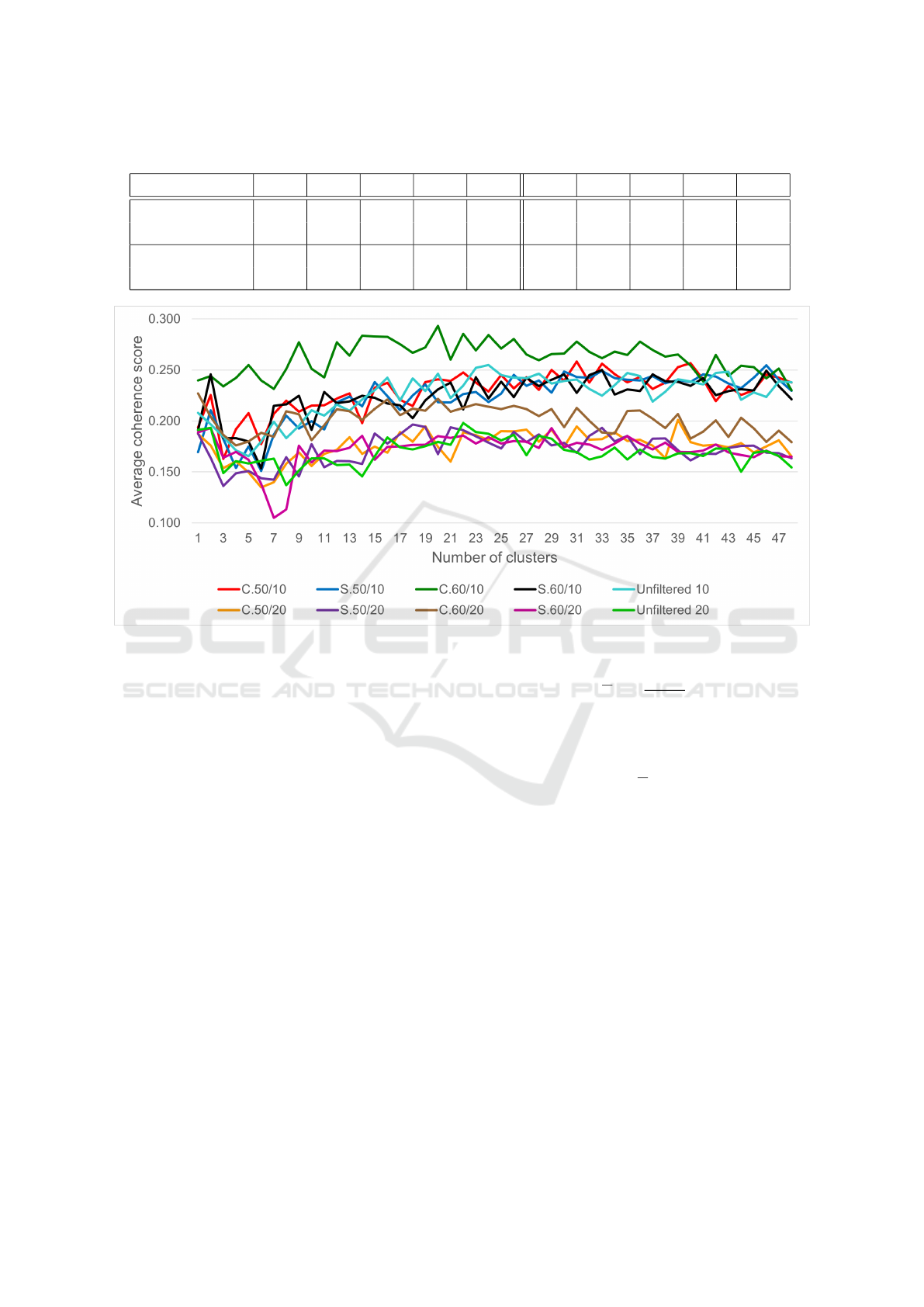
Table 1: Performance Summary.

Method C1 C2 S1 S2 U1 C3 C4 S3 S4 U2

Total Clusters 32 21 47 34 25 40 21 19 30 23

Mean Coherence 0.258 0.293 0.239 0.240 0.255 0.201 0.222 0.196 0.170 0.198

Viable Clusters 28 19 42 32 23 34 19 16 26 18

Mean Coherence 0.306 0.340 0.276 0.274 0.295 0.239 0.255 0.248 0.197 0.265

Figure 1: Mean cluster semantic coherence values as a function of cluster sizes for all 10 cases.

K is the number of clusters. The M most signiﬁcant

words in each VCD, d

, are then identiﬁed by calcu-

lating TF-IDF scores for all words in d

relative to all

the other VCDs.

Terms that occur with a disproportionately high

frequency in d

relative to the set D as a whole are

deemed as more signiﬁcant, and therefore more rep-

resentative of the cluster. These word TF-IDF values

are also used as weights in the cluster wordclouds.

Next, the pairwise cosine similarities between

vector space embeddings of all M signiﬁcant words

are calculated. The word embeddings used are

those given by the GloVe algorithm pre-trained on

Wikipedia data with 6 billion tokens and a 400,000

word vocabulary (Pennington et al., 2014) (down-

loaded from https://nlp.stanford.edu/projects/glove.)

A weighted average of these M(M −1)/2 cosine simi-

larities is then used as the cluster semantic coherence.

The weighting is necessary to suppress the role of

common words and amplify that of uncommon ones.

This is based on the frequency rank, r

, of the words,

, in the GloVe embedding database, where less fre-

quent words have a higher value (occur later in the

ranking). The weight for a word pair (w

) is cal-

culated as:

∑

p,q

(1)

where w

= (r

+ r

)/2. The coherence score Q

of a

cluster C

with VCD d

is then calculated as:

∑

j,k∈d

sim( j,k) (2)

where sim( j,k) is the cosine similarity between the

GloVe vectors of words w

and w

4 RESULTS AND DISCUSSION

To evaluate the approach described above, we applied

it to the corpus of US presidential speeches from Rea-

gan to Trump. These were chosen because: a) The

speeches are in modern English with no archaic us-

ages; and b) They cover a period that most readers

today would be familiar with, so the semantic quality

of clusters would be easier to determine.

Ten cases were considered as listed below :

1. Case C1: M = 10, Method C with θ

= 0.5.

2. Case C2: M = 10, Method C with θ

= 0.6.

Inferring Interpretable Semantic Cognitive Maps from Noisy Document Corpora

745

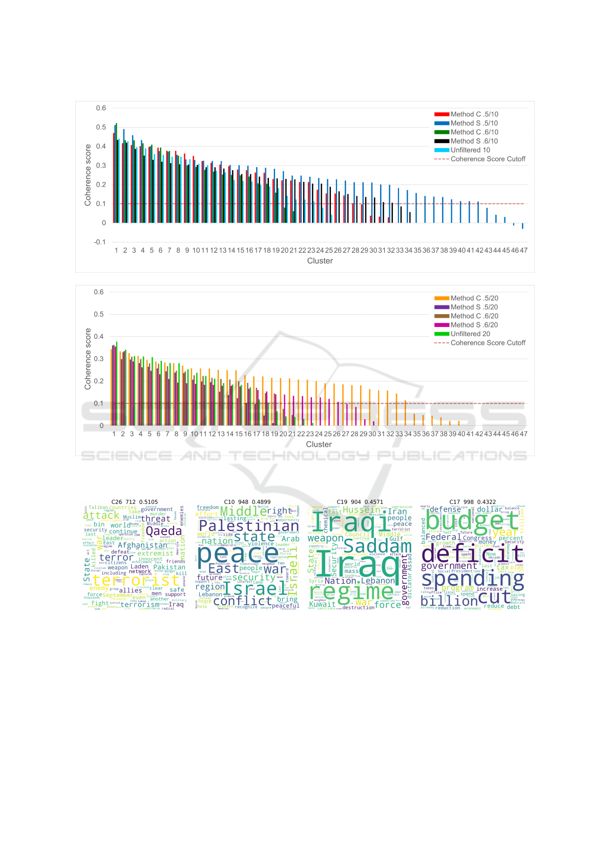
Figure 2: Rank plots of semantic coherence values for clusters. Top: M = 10 case; Bottom: M = 20 case. The horizontal red

line indicates a coherence value of 0.1 that is designated as the minimum necessary for a meaningful cluster (see text).

Figure 3: Wordclouds for the 4 most coherent clusters found in the S1 case. The legend at the top of each wordcloud indicates

cluster ID, cluster size, and the cluster semantic coherence value.

3. Case S1: M = 10, Method S matched with C1.

4. Case S2: M = 10, Method S matched with C2.

5. Case U1: M = 10, unﬁltered text.

6. Case C3: M = 20, Method C with θ

= 0.5.

7. Case C4: M = 20, Method C with θ

= 0.6.

8. Case S3: M = 20, Method S matched with C3.

9. Case S4: M = 20, Method S matched with C4.

10. Case U2: M = 20, unﬁltered text.

The quality of clustering depends signiﬁcantly on

both the θ

parameter (for the ﬁltered cases) and the

M parameter (for all cases, since M is used in deter-

mining the optimal cluster number in every case). Af-

ter exploring several values for each parameter, we

ICAART 2024 - 16th International Conference on Agents and Artiﬁcial Intelligence

746

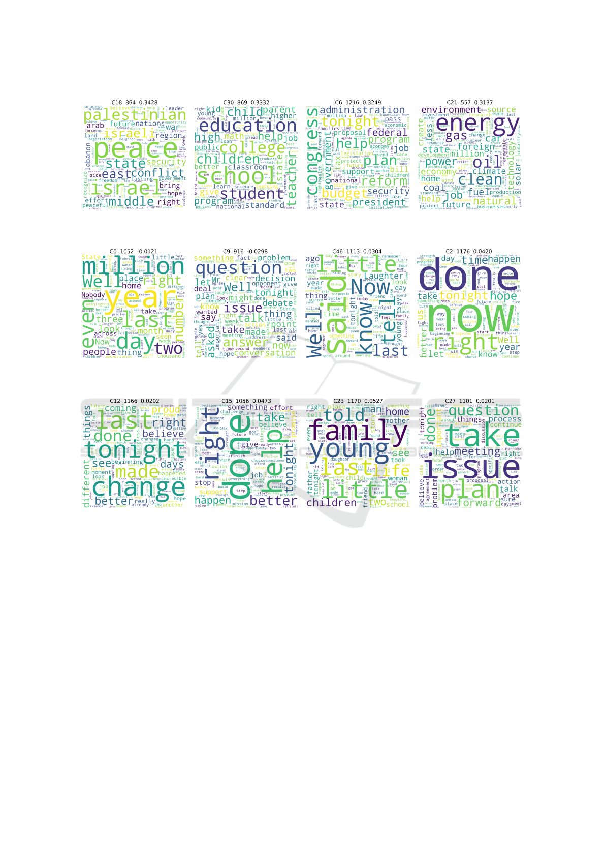
Figure 4: Wordclouds for the 4 most coherent clusters found in the C3 case. The legend at the top of each wordcloud indicates

cluster ID, cluster size, and the cluster semantic coherence value.

Figure 5: Wordclouds for the 4 least coherent clusters found in the S1 case. The legend at the top of each wordcloud indicates

cluster ID, cluster size, and the cluster semantic coherence value.

Figure 6: Wordclouds for the 4 least coherent C3 clusters that post-clustering ﬁltering at a coherence of 0.1 would remove.

The legend at the top of each wordcloud indicates cluster ID, cluster size, and the cluster semantic coherence value.

decided to use θ

values of 0.5 and 0.6, and M val-

ues of 10 and 20. A value θ

= 0.5 corresponds

roughly to 1.5 standard deviations below the mean,

while θ

= 0.6 is slightly above the mean. When com-

bined with the removal of short sentences, the 0.5 case

removes about 10% of all sentences (light ﬁltering),

while the 0.6 case removes about 60% (extreme ﬁlter-

ing). The goals are: a) To see if ﬁltering with either

or both methods produces better clusters than the cor-

responding unﬁltered cases; and b) Whether extreme

ﬁltering can help enhance performance.

Figure 1 shows the method for selecting the num-

ber of clusters in each of the 10 cases. Values of K

from 11 to 48 are considered. For each case, the mean

semantic coherence of the clusters found is plotted

against the number of clusters, K, and the K value

giving the highest mean coherence is chosen as the

number of clusters for that case. To keep compar-

isons fair, all clusterings are done using the same seed

value for centroid initialization in K-means cluster-

ing. This seed value is chosen empirically to be the

one that gives the least variance across cases. Across

the range of K, the mean coherence is much higher

for the C2 (M = 10, θ

= 0.6) case than for any other,

though the other methods catch up when K becomes

large. In general, using M = 20 reduces mean coher-

ence of clusters compared to the equivalent M = 10

case. This reﬂects the fact that using a higher M re-

sults in a more inclusive measure of coherence be-

cause it includes some less signiﬁcant words in the

Inferring Interpretable Semantic Cognitive Maps from Noisy Document Corpora

747

cluster. This tends to move the coherence values for

clusters somewhat closer because of an averaging ef-

fect. This is also why it is important to keep M limited

to a small value such as 10 or 20, and to evaluate the

M = 10 and M = 20 cases separately.

Table 1 shows how many clusters each method

produces at its optimal K (as determined from Fig-

ure 1), and the mean coherence of the clusters in each

case. It also shows how many clusters remain after

those with coherence below 0.1 are removed, and the

mean coherence of these viable clusters.

Figure 2 shows rank plots of cluster semantic co-

herence values obtained for all methods. The case

with the optimal number of clusters (based on Fig-

ure 1) is shown. The M = 10 and M = 20 cases are

plotted separately. The horizontal red line at a coher-

ence score of 0.1 indicates that clusters with coher-

ence value below this threshold are to be considered

of poor quality, and should be discarded. This repre-

sents an additional, post-clustering ﬁltering step. A

justiﬁcation for choosing 0.1 as the cutoff is that, as

Figure 1 shows, the mean cohesion of clusters across

all methods and K values stays above that level. Thus,

clusters with coherence below 0.1 can reasonably be

considered as falling below the worst-case mean.

For the M = 10 cases, the method giving the high-

est mean coherence in viable clusters is C2 (θ

= 0.6).

However, it produces only 19 viable clusters – prob-

ably because too many relevant sentences have been

ﬁltered away. C1, on the other hand, produces 28 vi-

able clusters with a good mean coherence of 0.307.

The largest number of viable clusters is produced by

S1 (42 clusters with a mean coherence of 0.276). S2

produces fewer clusters with lower mean coherence.

The unﬁltered case produces 23 viable clusters with

quite a good mean coherence of 0.295, but the 23rd

cluster for S1 is twice as coherent (Q = 0.241) as the

corresponding cluster of U1 (Q = 0.111). The 23rd

clusters of C1 and S2 are also much better. For the

M = 20 case, C3 (θ

= 0.5) is clearly the best. C4,

S3 and U2 produce few viable clusters, and S4 is also

dominated by C3 in both cluster number and mean

coherence. Thus, S1, C1 and C3 emerge as the best

options from this study. Figures 3 and 4 show the

wordclouds for the four most coherent clusters in the

S1 and C3 cases, respectively. For the same M value

in the coherence metric, a small amount of ﬁltering

(Cases C1, C3, S1, S3) produces a greater number

of coherent clusters than no ﬁltering (Cases U1 and

U2), though unﬁltered data can produce a few very

coherent clusters (C2). However, extreme ﬁltering

produces a lot fewer viable clusters.

One of the most interesting results to emerge from

the proposed method is the signiﬁcance of non-viable

clusters. Figures 5 and 6 shows the four least coherent

clusters produced by S1 and C3, respectively. All of

them are clearly dominated by rather generic terms,

and looking at the actual sentences in these clusters

conﬁrms that they have indeed swept up a large num-

ber of low relevance sentences that the other two ﬁl-

tering stages had left in the corpus. Thus, the clus-

tering process can itself be seen as a third stage of

relevance ﬁltering.

It is also notable that the lightly ﬁltered cases

(C1, C3, S1, S3) identify more removable clusters

than the unﬁltered case, even though the unﬁltered

data has many more removable sentences. This im-

plies that the unﬁltered clustering is smearing seman-

tic noise across some or all of its viable clusters, but

pre-ﬁltering is removing some of it, allowing the clus-

tering process to squeeze out still more.

The results for both the best and worst clusters

also show that the coherence metric used in this study

is meaningful, and correlates well with human judge-

ments of coherence. A more systematic study of this

with human evaluators will be reported in future pa-

pers.

5 CONCLUSION

The primary conclusion from this study is that the

method described can produce good, interpretable,

domain-speciﬁc semantic cognitive maps from cor-

pora of long, real-world documents with semantic

noise. As a side-effect, the method also provides an

effective way of removing irrelevant text from doc-

uments, both through pre-ﬁltering and further post-

clustering ﬁltering. The wordclouds of the low co-

herence clusters obtained and removed show that

they perform a “garbage collection” function. The

very simple, purely lexical heuristic relevance ﬁlter-

ing method we tried (Method S) performed well, with

the S1 case producing the largest number of viable

clusters with a high mean coherence value, and S2

also performing well. Filtering with Method C gave

fewer, though higher-quality, clusters in the M = 10

case. The results in the M = 20 case were more am-

biguous, and produced fewer viable clusters. Future

work includes looking at varying the viability thresh-

old, applying the method to even noisier corpora, and

integrating it into an automated discussion tracking

and guidance system.

ICAART 2024 - 16th International Conference on Agents and Artiﬁcial Intelligence

748

ACKNOWLEDGEMENTS

This work was partially supported by Army Research

Ofﬁce Grant No. W911NF-20-1-0213.

REFERENCES

Beltagy, I., Peters, M. E., and Cohan, A. (2020). Long-

former: The long-document transformer. arXiv

preprint arXiv:2004.05150.

Cer, D., Yang, Y., Kong, S.-Y., Hua, N., Limtiaco, N.,

St. John, R., Constant, N., Guajardo-Cespedes, M.,

Yuan, S., Tar, C., Strope, B., and Kurzweil, R. (2018).

Universal sentence encoder for English. In Proceed-

ings of the 2018 Conference on Empirical Methods

in Natural Language Processing: System Demonstra-

tions, pages 169–174, Brussels, Belgium. Association

for Computational Linguistics.

Choudhary, R., Alsayed, O., Doboli, S., and Minai, A.

(2022). Building semantic cognitive maps with text

embedding and clustering. In 2022 International Joint

Conference on Neural Networks (IJCNN), pages 01–

08. IEEE.

Choudhary, R., Doboli, S., and Minai, A. A. (2021). A

comparative study of methods for visualizable se-

mantic embedding of small text corpora. In 2021

International Joint Conference on Neural Networks

(IJCNN’21), pages 1–8. IEEE.

Conneau, A., Kiela, D., Schwenk, H., Barrault, L., and

Bordes, A. (2017). Supervised learning of universal

sentence representations from natural language infer-

ence data. In Proceedings of the 2017 Conference on

Empirical Methods in Natural Language Processing,

pages 670–680, Copenhagen, Denmark. Association

for Computational Linguistics.

Coursey, L., Gertner, R., Williams, B., Kenworthy, J.,

Paulus, P., and Doboli, S. (2019). Linking the di-

vergent and convergent processes of collaborative cre-

ativity: The impact of expertise levels and elaboration

processes. Frontiers in Psychology, 10:699.

Devlin, J., Chang, M.-W., Lee, K., and Toutanova, K.

(2019). BERT: Pre-training of deep bidirectional

transformers for language understanding. In Proceed-

ings of the 2019 Conference of the North American

Chapter of the Association for Computational Lin-

guistics: Human Language Technologies, Volume 1

(Long and Short Papers), pages 4171–4186, Strouds-

burg, PA, USA. Association for Computational Lin-

guistics.

Fisher, D., Choudhary, R., Alsayed, O., Doboli, S., and Mi-

nai, A. (2022). A real-time semantic model for rele-

vance and novelty detection from group messages. In

2022 International Joint Conference on Neural Net-

works (IJCNN), pages 01–08. IEEE.

Jones, K. S. (1972). A statistical interpretation of term

speciﬁcity and its application in retrieval. Journal of

Documentation, 28:11–21.

Kuan, J. and Mueller, J. (2022). Back to the basics: Revis-

iting out-of-distribution detection baselines. In 2022

ICML Workshop on Principles of Distribution Shift.

Lample, G. and Conneau, A. (2019). Cross-lingual

language model pretraining. arXiv preprint

arXiv:1901.07291.

Le, Q. and Mikolov, T. (2014). Distributed representations

of sentences and documents. In Xing, E. P. and Je-

bara, T., editors, Proceedings of the 31st International

Conference on Machine Learning, volume 32 of Pro-

ceedings of Machine Learning Research, pages 1188–

1196, Bejing, China. PMLR.

Lilleberg, J. (2020). United states presidential

speeches. https://www.kaggle.com/datasets/littleotter/

united-states-presidential-speeches. Accessed:2023.

Lo, K., Jin, Y., Tan, W., Liu, M., Du, L., and Buntine,

W. (2021). Transformer over pre-trained transformer

for neural text segmentation with enhanced topic co-

herence. In Findings of the Association for Com-

putational Linguistics: EMNLP 2021, pages 3334–

3340, Punta Cana, Dominican Republic. Association

for Computational Linguistics.

Luhn, H. P. (1957). A statistical approach to mechanized

encoding and searching of literary information. IBM

Journal 1(4), pages 309–317.

Mikolov, T., Chen, K., Corrado, G., and Dean, J. (2013).

Efﬁcient estimation of word representations in vec-

tor space. In Bengio, Y. and LeCun, Y., editors,

1st International Conference on Learning Represen-

tations, ICLR 2013, Scottsdale, Arizona, USA, Work-

shop Track Proceedings.

OpenAI (2023a). ChatGPT: Optimizing language models

for dialogue.

OpenAI (2023b). GPT-4 technical report.

Pang, B., Nijkamp, E., Kry

sci

nski, W., Savarese, S., Zhou,

Y., and Xiong, C. (2022). Long document summariza-

tion with top-down and bottom-up inference. arXiv

preprint arXiv:2203.07586.

Pennington, J., Socher, R., and Manning, C. (2014). GloVe:

Global vectors for word representation. In Proceed-

ings of the Conference on Empirical Methods in Nat-

ural Language Processing (EMNLP), pages 1532–

1543.

Reimers, N. and Gurevych, I. (2019). Sentence-BERT:

Sentence embeddings using siamese BERT-networks.

In Proceedings of the 2019 Conference on Empiri-

cal Methods in Natural Language Processing, page

3982–3992.

Song, K., Tan, X., Qin, T., Lu, J., and Liu, T.-Y. (2020). MP-

net: Masked and permuted pre-training for language

understanding. Advances in Neural Information Pro-

cessing Systems, 33:16857–16867.

Tatman, R. (2017). Google web trillion word corpus. https:

//www.kaggle.com/rtatman/english-word-frequency.

Accessed:2021.

Tolman, E. C. (1948). Cognitive maps in rats and men. Psy-

chological Review, 55:189–208.

Inferring Interpretable Semantic Cognitive Maps from Noisy Document Corpora

749