Automatic Registration of 3D Point Cloud Sequences

Nat

alie V

ıtov

, Jakub Frank and Libor V

Department of Computer Science And Engineering, Faculty of Applied Sciences, University of West Bohemia,

Univerzitn

ı 8, 301 00 Plze

n, Czech Republic

Keywords:

Registration, Point Cloud, Dynamic, Series, Kinect, Sensor, Alignment.

Abstract:

Surface registration is a well-studied problem in computer graphics and triangle mesh processing.

A plethora of approaches exists that align a partial 3D view of a surface to another, which is a central task

in 3D scanning, where usually each scan only provides partial information about the shape of the scanned

object due to occlusion. In this paper, we address a slightly different problem: a pair of depth cameras is

observing a dynamic scene, each providing a sequence of partial scans. The scanning devices are assumed to

remain in a constant relative position throughout the process, and therefore there exists a single rigid trans-

formation that aligns the two sequences of partial meshes. Our objective is to ﬁnd this transformation based

on the data alone, i.e. without using any specialized calibration tools. This problem can be approached as

a set of static mesh registration problems; however, such an interpretation leads to problems when enforcing

a single global solution. We show that an appropriate modiﬁcation of a previously proposed consensus-based

registration algorithm is a more viable solution that exploits information from all the frames simultaneously

and naturally leads to a single global solution.

1 INTRODUCTION

Depth cameras, both time-of-ﬂight- and structured-

light-based, are popular tools for obtaining informa-

tion about a 3D shape. Devices such as various ver-

sions of Microsoft Kinect or Intel RealSense provide

a depth map, where each pixel represents a depth mea-

surement—its intensity is related to the distance from

the device to the nearest surface. However, even in

ideal conditions, such data is insufﬁcient for scanning

even simple shapes due to self-occlusion. When con-

structing a full model, the scanning device is typi-

cally moved around, capturing the shape from vari-

ous points of view, or the object itself is moved, po-

tentially using a turntable, to acquire multiple par-

tial views that can be combined into a single, com-

plete model. The process of ﬁnding the rigid transfor-

mations that transform the partial scans into a single

global coordinate system is known as registration.

However, this approach cannot be applied when

the object being captured is dynamic. In such a case,

it is possible to use multiple scanning devices, each

covering a part of the surface. If these devices work

at the same frame rate and are synchronized, corre-

https://orcid.org/0009-0009-4596-1271

https://orcid.org/0000-0002-0213-3769

sponding frames can be aligned and form a more com-

plete view of the scene than each separately. How-

ever, due to the dynamic nature of the data, frames

captured at different time instants cannot be aligned

since they capture a different shape, in general. On

the other hand, as long as the capture devices remain

at a constant relative position, the solution to the reg-

istration problem should remain constant for each pair

(or set) of partial meshes captured at the same time in-

stant. This, in turn, can and should be used when ﬁnd-

ing the transformation: the solution should align all

the frames where non-ambiguous shape matches are

present. When shapes match ambiguously or poorly

in a certain frame, information from the other frames

can be used to resolve the ambiguity.

Our primary focus is on applying virtual reality

in physiotherapy, speciﬁcally for patients with condi-

tions like multiple sclerosis. In this context, patients

perform exercises in a virtual environment, evaluated

in real-time using trackers. These exercises, rooted

in proprioceptive neuromuscular facilitation (Moreira

et al., 2017), involve seated upper limb movements in

a diagonal direction. To demonstrate the exercises ef-

fectively, we aim to show patients a 3D recording of

the ideal performance, captured with a 3D acquisition

device (Microsoft Kinect for Azure). However, a sin-

Vítová, N., Frank, J. and Váša, L.

Automatic Registration of 3D Point Cloud Sequences.

DOI: 10.5220/0012388400003660

Paper published under CC license (CC BY-NC-ND 4.0)

In Proceedings of the 19th International Joint Conference on Computer Vision, Imaging and Computer Graphics Theory and Applications (VISIGRAPP 2024) - Volume 1: GRAPP, HUCAPP

and IVAPP, pages 261-268

ISBN: 978-989-758-679-8; ISSN: 2184-4321

261

gle viewpoint provides insufﬁcient data, prompting us

to seek a setup that captures at least two points of view

and merges the data into a comprehensive stream of

point clouds.

While temporal synchronization is easily

achieved, spatial alignment of the partial streams

poses a challenge. We strive for a user-friendly

setup for therapists, avoiding complex calibration and

allowing automatic data merging. Our approach mod-

iﬁes an existing static mesh registration algorithm,

enabling natural alignment of point cloud sequences.

The resulting tool is versatile, robust, fully automatic,

and generates a single aligning transformation based

on information from all frames, excluding those with

limited reliable information.

2 RELATED WORK

The challenge of registering 3D shapes — aligning

their overlapping parts through a rigid orientation-

preserving transformation (known as a special orthog-

onal transformation, SO(3)) — is a well-studied prob-

lem. It arises not only in completing partial scans

but also in areas like motion analysis, scene analy-

sis, object identiﬁcation, and retrieval. While the hu-

man brain ﬁnds the problem essentially easy, being

trained to match 3D shapes, constructing a reliable

and fast computer algorithm for this problem proves

to be rather difﬁcult. This difﬁculty stems from the di-

mension of the solution space (6D), which prohibits

efﬁcient brute-force methods, and the general chal-

lenge of representing the naturally understood con-

cept of (even local) shape similarity while working

with the most common shape representations like tri-

angle meshes or point clouds.

Out of the plethora of algorithms, we mention

a few that are relevant to this work (for a comprehen-

sive overview, refer to (Castellani and Bartoli, 2020)).

Algorithms can generally be local, starting with some

initial relative position of the input shapes and iter-

atively improving their alignment, or global, ﬁnding

an aligning transformation independently of the initial

relative position of the inputs. A popular local tech-

nique is the Iterative Closest Point algorithm (ICP),

which alternates between estimating correspondences

and ﬁnding the optimal rigid transformation that best

aligns the correspondence pairs in the sense of the

sum of squared distances. Note that the last task can

be solved in closed form using the Kabsch algorithm

(Kabsch, 1976).

Later, the ICP approach has been improved in var-

ious ways, focusing on aspects like pruning corre-

spondences or using different objectives for the op-

timal rigid transformation step. In particular, various

norms have been investigated in the work of (Bouaziz

et al., 2013), yielding an algorithm that is claimed to

perform on par with global registration algorithms.

Another similar borderline approach has been pro-

posed by (Zhou et al., 2016). It uses the Fast Point

Feature Histogram (FPFH, proposed by (Rusu et al.,

2009)) features that are matched, and a subset of valid

matching pairs is iteratively reﬁned, using an objec-

tive function that smoothly transits from global to lo-

cal matching.

Fully global approaches usually rely on identify-

ing speciﬁc shape features in the pair of shapes be-

ing aligned. These may include a quadruple of points

in a certain conﬁguration, used by algorithms like

4pcs (Aiger et al., 2008) or Super4pcs (Mellado et al.,

2014), or a local curvature-based descriptor used by

the RANSAC algorithm proposed by (Hruda et al.,

2019). The latter serves as the basis on which our

registration for dynamic point clouds is build, thus it

is described in more detail in 3.2.

All algorithms mentioned are primarily targeted

at registering static triangle meshes. Several ways ex-

tend this task to a ”dynamic” setting, such as combin-

ing shape and color information (Bouaziz and Pauly,

2013), scanning a static object with a moving camera

(Weber et al., 2015; He et al., 2018), or dealing with

a deforming object (Mitra et al., 2007). Articulated

shapes are explored by (Chang and Zwicker, 2008).

None of these interpretations of ”dynamic” matches

our objective.

Our work relates more closely to the problem of

(semi-)automatic calibration of 3D scanning devices.

Here, the task is also ﬁnding a rigid transformation to

bring data captured by one sensor into the coordinate

frame of another. However, the tools used for this task

are usually different from the ones we wish to use:

typically, a custom apparatus, such as a checkerboard

pattern in (Raposo et al., 2013a; Raposo et al., 2013b),

a colored sphere in (Fornaser et al., 2017), or a partic-

ular human pose as proposed by (Eichler et al., 2022),

is used in the pre-capture stage. The camera/sensor

setup is then deemed calibrated until the devices are

moved, using the results of the preprocessing step to

bring the inputs into alignment. However, our objec-

tive is to eliminate the need for a dedicated calibration

stage and the risk of calibration loss that may occur

before actual acquisition.

GRAPP 2024 - 19th International Conference on Computer Graphics Theory and Applications

262

3 REGISTRATION ALGORITHM

DESCRIPTION

In this section, we ﬁrst formalize the input and ob-

jective. Then we provide a basic overview of the

RANSAC-based static mesh registration algorithm, as

needed to understand the last subsection, where our

registration algorithm for point cloud sequences will

be presented.

3.1 Input, Objective

The input data consist of two sequences P =

, P

, ..., P

) and Q = (Q

, Q

, ..., Q

) of point

clouds P

= (p

, p

, ..., p

), Q

= (q

, q

, ..., q

where each point cloud (also called a frame) consists

of a set of points. Each p

and q

is a three com-

ponent vector of the Cartesian coordinates of the j-th

point of the i-th frame of P and Q , respectively. Both

P and Q have the same number n of frames, but each

frame in P and Q has a potentially different number

of points m

and m

, respectively.

The sequences are synchronized, i.e., each Q

has

been captured at the same time instant as P

; how-

ever, each has been captured by a different depth sen-

sor, and thus each captures a different portion of the

scene, and crucially, each set of points is represented

in a local coordinate frame of its depth sensor. There-

fore, even though large parts of the scene are captured

in both sequences (although not necessarily in all the

frames), these overlapping parts are not aligned. The

objective is to ﬁnd a single rigid transformation T , s.t.

when applied to each frame Q

, i.e., to all of its ver-

tices, it produces a transformed frame T (Q

), where

the areas of captured overlap coincide with their coun-

terpart in P

3.2 Registration of Static Meshes

A general framework for Random Sample Consensus

(RANSAC) registration of static meshes has been pro-

posed by (Hruda et al., 2019). Our registration algo-

rithm builds on the concepts used in their work, and

therefore we review the most important steps of their

approach here. For a detailed description and justiﬁ-

cation of each step, please refer to the original paper.

The objective is similar to that outlined in the pre-

vious section, only this time working with a pair of

meshes P and Q: the task is to ﬁnd a transforma-

tion T , s.t. T (Q) brings overlap in Q into alignment

with corresponding parts of P. First, surface normals

are estimated for all vertices of P and Q. The algo-

rithm then continues by sampling both input meshes

on a quasi-regular grid. A set of surface samples on

P is built, covering its surface uniformly. For each

sample point, the principal curvatures are estimated

and stored, together with the ﬁrst principal curvature

direction.

Next, Q is sampled in a similar fashion. For each

sample q

on Q, the principal curvatures are estimated

as well, and the most similar point p

in the set of sam-

ples from P in terms of curvature estimates is found

using a KD-tree data structure. Having a point on Q

and a potentially corresponding point on P, it is pos-

sible to build a pair of candidate transformations T

and T

−

by building the unique pair of rigid transfor-

mations such that

1. T (q

) = p

2. the transformed normal of q

aligns with the nor-

mal of p

3. the transformed ﬁrst principal curvature direction

of q

aligns with the ﬁrst principal curvature di-

rection of p

(for T

) or its opposite direction (for

−

By sampling the vertices of the mesh Q, a set of

predeﬁned size (10 000 by default) of such candi-

date transformations is built, where each transforma-

tion must pass a veriﬁcation test: a subsampled ver-

sion of the mesh Q is transformed by each T

, and

the size of the resulting overlap is estimated by eval-

uating the proportion of vertices of T

(Q), which lie

in close proximity to vertices of the mesh P. The re-

quired proximity and the ratio required to pass the test

are also conﬁgurable parameters.

The key observation for the ﬁnal step of the al-

gorithm is that in the set of candidate transforma-

tions, many are wrong; however, many others are

close to the correct solution. These transformations,

in turn, form a high-density cluster in the 6D space

of rigid transformations, in which all the candidate

transformations live. The key ingredient required for

ﬁnding this density peak is an appropriate notion of

transformation similarity. Hruda et al. discuss vari-

ous choices and conclude that transformation distance

cannot be evaluated without taking into account the

data on which the transformations are applied. For

the application at hand, it is straightforward that the

transformations are applied to the vertices of Q, and

thus the difference (i.e., dissimilarity, distance) of two

candidate transformations T

and T

can be expressed

as:

d(T

, T

) =

∑

i=0

∥T

) − T

)∥, (1)

where m

is the number of vertices in Q and q

are

the vertices of Q. Even though this formulation of the

distance seems to require evaluating a sum over all

the vertices of Q (i.e., linear complexity w.r.t. m

), it

Automatic Registration of 3D Point Cloud Sequences

263

can be shown that with pre-processing, this distance

can, in fact, be evaluated in constant time (see (Hruda

et al., 2019) for details), and thus it can be evalu-

ated repeatedly without affecting the overall runtime

of the algorithm dramatically, even for complex input

meshes P and Q.

Having the notion of distance, it is ﬁnally easy

to estimate the density of the set of candidate trans-

formations around a particular candidate as a sum of

gaussians:

ρ(T

) =

∑

∈T

exp(−(σ d(T

, T

))

), (2)

where T is the set of all constructed candidate trans-

formations, and σ is a user-speciﬁed parameter that

controls the smoothness of the estimated density func-

tion. The candidate with the largest ρ(T

) is ﬁnally

selected as the solution to the problem.

This algorithm, initially designed for aligning

static meshes, could be adapted for dynamic point

clouds by applying it to individual frames. In fact,

any other method for static mesh registration can be

used this way. However, this results in a sequence of

diverse solutions rather than a single answer. Using

transformation blending to merge single-frame align-

ing transformations poses challenges, including po-

tential difﬁculties in registering some frames and the

risk of outliers affecting the overall alignment accu-

racy. Instead, we propose modifying the registration

algorithm to naturally accept two sequences of point

clouds, considering all frames and ensuring simulta-

neous alignment while diminishing the inﬂuence of

frames with insufﬁcient reliable information. We con-

tend that the algorithm by Hruda et al. is well-suited

for this extension. The subsequent subsection pro-

vides a detailed description of this extension.

3.3 Registration of Dynamic Point

Clouds

There are two main differences between the original

method and the one we are proposing here. First,

we are working with point clouds instead of triangle

meshes, and second, the inputs are sequences instead

of just one frame. The ﬁrst change mainly affects

the estimation of normals and curvatures, whereas the

second one affects major parts of the algorithm, such

as the accumulation of candidates, their veriﬁcation,

and the identiﬁcation of the ﬁnal solution.

3.3.1 Estimation of Normals

In our algorithm, we estimate normals in point clouds

by ﬁtting the points nearest to a given point with

a plane in the least squares sense, declaring the

plane’s normal as the estimated normal at that point.

A KD-tree structure is employed for ﬁnding a set of

closest points, with a dynamic radius adjustment to

address non-uniform point distribution - the KD-tree

searches for the points in a given radius, and if the

number of points found does not ﬁt in a preset inter-

val, the radius is modiﬁed. Isolated points are dis-

carded, and for non-isolated ones, the normal is cal-

culated as the least squares ﬁt to the vectors from each

neighbor to the centroid. To ensure consistent orien-

tation, normals pointing away from the camera are

ﬂipped based on the relationship n · p < 0, where n

is the normal and p is vector of point coordinates in

the coordinate system of the device.

For the experiments presented below, we required

between 15 to 30 neighboring points, starting with an

initial search radius of 8mm. If more points than 30 is

found, then the radius is reduced by multiplication by

0.8. Should the opposite case occur, with fewer than

15 points found, the radius is multiplied by 1.2. If

a distance of 300mm is reached, and fewer than three

points were found, the point is considered isolated.

These constants were found experimentally for our

data. Since the radius from previous successful search

is used in each subsequent search, the normal estima-

tion involves only 1.09 KD-tree queries per vertex on

average.

3.3.2 Estimation of Curvature

For curvature estimation, the KD-tree structure re-

places the original breadth-ﬁrst-search of connectivity

in (Hruda et al., 2019) for ﬁnding the closest points

around the investigated one. The search runs with

a ﬁxed radius, crucial for consistent curvature estima-

tion, which can be set based on data character. In the

local point cloud, which consists of the nearest points

found, a basis aligned with normal/tangent directions

is built, and curvatures are estimated using a 2x2 sym-

metric matrix. Using a Gaussian kernel, weights re-

ﬂecting neighbor distances are assigned to each point,

with the center having the weight of 1.

The eigenvalues of the constructed matrix repre-

sent principal curvatures, with eigenvectors indicat-

ing principal curvature directions in the tangential

plane. Converting eigenvectors into local coordinates

provides principal curvature directions in the model

space.

After estimating point cloud normals and sam-

pling data, candidate transformations are built for

each corresponding frame pair and are later pooled

into a single set of candidate transformations. Unlike

the original method, our algorithm skips the veriﬁ-

cation test to avoid excessive memory requirements.

GRAPP 2024 - 19th International Conference on Computer Graphics Theory and Applications

264

Instead, we propose curvature-based ﬁltering. Differ-

ences in curvatures between corresponding points are

stored, and candidates are ﬁltered based on this score:

a certain percentage of candidates where the differ-

ence is highest is discarded from further processing.

This approach improves computational efﬁciency and

robustnes of the algorithm.

The transformation between input sequences is

found as the density peak in the space of candidate

transformations. This ﬂexible approach works on se-

quences or single frame pairs, and on point clouds

or meshes. Evaluating candidate transformation dis-

similarity (Eq. 1) considers the entire sequence Q

rather than a single frame. This only affects the pre-

processing phase, with the actual evaluation of trans-

formation dissimilarity independent of frame count or

point density in the frames.

4 EXPERIMENTAL RESULTS

We have tested the proposed algorithm on a set of re-

alistic data, acquired by a pair of depth cameras. In

section 4.1, we describe the character of the test data,

and in section 4.2, we describe the quantitative results

of our experiments.

4.1 Data Acquisition

The objective of registering dynamic point clouds

originates from a rehabilitation application designed

for multiple sclerosis patients. In this virtual reality

therapy, patients, wearing HTC Vive headsets, are im-

mersed in a virtual environment without visual cues

from the real world. The goal is to provide a 3D ani-

mation of therapists movements, enhancing the exer-

cise experience.

Two Microsoft Kinect for Azure devices were

chosen for recording due to their affordability and

synchronization capabilities. Operating in depth

mode with a resolution of 640x526 points and 30

frames per second, these devices capture depth maps,

converted into point clouds using the Kinect for

Azure SDK. Synchronization between the devices is

achieved using a 3.5mm jack cable, ensuring tempo-

ral alignment of recorded scenes. The synchronized

sequences are saved as *.obj ﬁles for further process-

ing.

For the testing of our algorithm, we recorded sev-

eral scenes. In each case, we attempted to achieve

a certain known relative position of the sensors; how-

ever, due to the limited precision of manual placement

of the devices, this was likely achieved only approxi-

mately. The following datasets were acquired:

Table 1: Frame counts (#F) and average point counts (#P)

of the used datasets.

dataset #F #P principal #P agent

static 351 261942 258726

left-diag 266 262508 260575

right-diag 247 261658 254731

translate 285 266432 261150

• static represents a scene without any actors. The

devices were placed 100 cm apart horizontally,

and both faced one point at a distance of 151.5cm

from the baseline.

• left-diag represents the left diagonal from PNF

methodology, using devices shifted by 100cm and

both facing one point distant 151.5cm.

• right-diag represents the right diagonal from PNF

methodology using devices shifted by 100cm and

both facing one point distant 151.5cm.

• translate represents the left PNF diagonal with

both devices facing the same direction with the

separation of devices by 50cm.

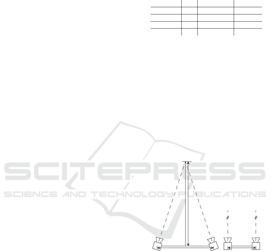
The conﬁgurations are also shown in Figure 1. The

frame counts and average point counts are listed in

Table 1.

principal

device

agent

device

100 cm

151.5 cm

principal

device

agent

device

50 cm

Figure 1: Conﬁguration of devices used for acquisition of

test data. On the left, conﬁguration used for the static, left-

diag and right-diag datasets, on the right the conﬁguration

used for the translate dataset.

4.2 Experiments

To validate the proposed method, we utilised the de-

scribed datasets. Figure 2 illustrates a frame from

the left-diag dataset, showcasing both the source se-

quence (agent device) and the target sequence (princi-

pal device). Despite having information about the in-

tended relative placement of the two sensors used for

data acquisition, this information is only approximate

Automatic Registration of 3D Point Cloud Sequences

265

and cannot be treated as a ground truth transforma-

tion from one sensor to the other. We manually con-

structed the transformation based on measured dis-

tances between sensors and the object (see to Fig-

ure 1), denoted as design transformation. While this

transformation should closely match the true align-

ing transformation, imperfections arise due to impre-

cise manual measurements and potential internal bias

from the devices, resulting in an imperfect transfor-

mation upon visual evaluation.

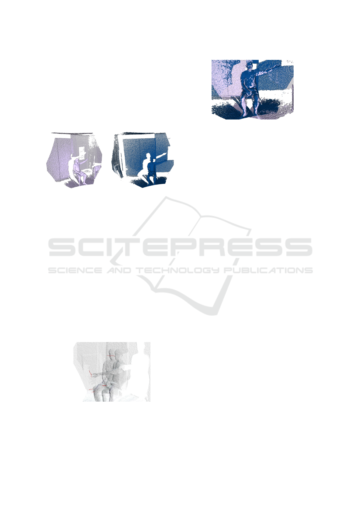
Figure 2: Source (left) and target (right) data from the left-

diag dataset. The colours are kept the same for other pic-

tures so the source and target are distinguished.

Since the design transformation cannot be used to

determine the degree of correctness of the ﬁnal com-

puted transformation, we have constructed a differ-

ent manual transformation and consider it our artiﬁ-

cial ground truth. To build this transformation, we

have manually selected four matching points from

one frame pair and using the Kabsch algorithm, we

have constructed a transformation, which will be re-

ferred to as the manual transformation. To ensure

the manual transformation is as close to the ground

truth as possible, we have selected easily recognized

points - nose tip, ﬁngertip of the left hand, right knee

and a knuckle of the right hand. These points are

shown in Figure 3. The result of merging the source

transformed by the manual transformation and the tar-

get is shown in Figure 4, and after visual assessment

we consider this transformation better than the design

transformation.

Figure 3: Points selected for the Kabsch algorithm are high-

lighted with red vectors. Easily recognized points were

chosen: nose tip, ﬁngertip on the left hand, right knee and

a knuckle on the right hand (left-diag dataset, frame 210).

Figure 4: Source transformed by the manual transformation

compared to the target (left-diag dataset).

Several parameters inﬂuence the algorithm’s

speed and accuracy, measured as the difference be-

tween the computed transformation and the manual

transformation. To calculate this difference, we trans-

form a point cloud with both transformations and cal-

culate the mean distance between corresponding point

pairs for all the transformed vertices across all frames.

This in turn allows us to assign the ﬁnal result a unit:

it can be interpreted as the average distance of each

point in each point cloud from its optimal position as

induced by the reference transformation.

The algorithm’s parameters include the number

of frames, the number of constructed candidates for

each frame, the percentage of candidates preserved

after ﬁltering, the radius used for collecting neighbors

when estimating curvatures, and the shape parameter

for the Gaussian kernel used for weighting them in

Eq. 2.

We designed and run several experiments to prop-

erly set different parameters. One of them aimed to

determine the sufﬁcient number of frames and candi-

date transformations that yield robust results without

incurring unnecessary computational overhead from

using the complete set of frames. Our objective was

to use the minimum number of candidate transfor-

mations for density calculation, selecting only a cer-

tain percentage of input frames to cancel out noise

in the data. Empirically, we have veriﬁed that a total

of 2 000 000 constructed candidate transformations, of

which 1% is preserved through ﬁltering, leads to a ro-

bust registration for all our test datasets.

Finally, we have compared the transformation

computed using the parameters from the two previous

experiments to the manual transformation and visu-

ally assessed the resulting merge of the transformed

source with the target. Figure 5 illustrates the results

of the registration experiment across all datasets.

The remaining parameters were set as follows: We

selected 100 consecutive frames from the middle part

of the input sequence. In the case of the left-diag

dataset, these frames depict the actor’s arm moving ei-

ther up or down on the diagonal. Choosing the middle

part helped avoid static frames from both the begin-

GRAPP 2024 - 19th International Conference on Computer Graphics Theory and Applications

266

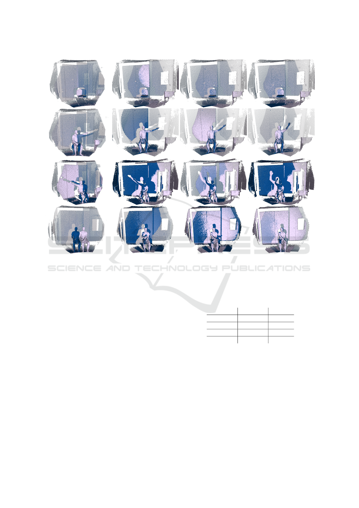
Figure 5: The results of the registration process for all datasets are presented, arranged from top to bottom as follows:

static, left-diagonal, right-diagonal, and translate. The leftmost column displays the original data without any modiﬁcations.

Subsequent columns present the source point cloud after the transformation together with the target point cloud. The frames

are displayed in their chronological order, with a 10-frame interval, to show visible changes between frames. Our registration

algorithm was applied to each dataset separately, yielding transformations from 100 frames of data.

ning and end of the sequence, ensuring that all frames

captured dynamic arm movement. To test the algo-

rithm’s robustness, data were not preprocessed, and

the noise, mainly in the background, remained part of

the original data without alterations.

The average difference between the resulting

transformation and the manual transformation, along

with the algorithm’s running times, is summarized

in Table 2. The performance has been measured on

a PC with AMD Ryzen 3950X CPU and 32GB of

RAM, using a reference implementation written in the

C# language. While optimizing the process is feasible

with a more performance-oriented programming lan-

guage, the current performance sufﬁces for our prac-

tical application since registration is a one-time oper-

ation for each new exercise. It is worth noting that

differences in the order of centimeters can be con-

sidered successful, given the overall scale of the cap-

tured point clouds is in the order of several meters

and considering the overall level of noise produces by

Table 2: Differences from manual transformation (diff) and

computation times for all datasets.

dataset diff [mm] time [s]

static 45.37 165.9

left-diag 52.17 170.2

right-diag 120.73 175.4

translate 107.44 177.0

the sensors. Additionally, the manual transformation

may also have inherent biases w.r.t. the true aligning

transformation.

5 CONCLUSIONS

We have presented an algorithm for the automatic reg-

istration of point cloud sequences. This algorithm

builds on a speciﬁc static mesh registration algorithm

chosen for its beneﬁcial properties. Notably, it en-

ables us to elegantly incorporate information from all

Automatic Registration of 3D Point Cloud Sequences

267

frames, constructing and ﬁltering a global pool of can-

didate transformations. In this pool, the ﬁnal, single

solution is determined by identifying the density peak

in the space of rigid transformations. The distance

metric used is derived from the knowledge of the en-

tire dataset undergoing transformation – in our case,

it is the set of all points from all input frames.

The algorithm delivers robust results, even when

applied to noisy data acquired by current consumer-

grade depth sensors. Speciﬁcally, we have used the

algorithm to align four sequences captured with a pair

of Microsoft Kinect for Azure devices. In each in-

stance, the resulting transformation closely matched

the expected result, offering visually superior results

compared to aligning the data based on the relative

placement information of the input devices.

In the future, we intend to explore more advanced

local shape descriptors than those used in this work.

Enhancing our understanding of local shape matching

could result in improved candidate transformation ﬁl-

tering, leading to a faster and more reliable algorithm.

A reference implementation of the proposed

registration tool is available for download at

https://github.com/natvitova/DynamicRegistration.

ACKNOWLEDGEMENTS

This work was supported by the project 20-02154S

of the Czech Science Foundation. Nat

alie V

ıtov

and Jakub Frank were partially supported by the Uni-

versity speciﬁc research project SGS-2022-015, New

Methods for Medical, Spatial and Communication

Data. The work was partially carried out as part of

the study ”Virtual reality in the physiotherapy of mul-

tiple sclerosis” supported by GAUK 202322.

REFERENCES

Aiger, D., Mitra, N. J., and Cohen-Or, D. (2008). 4-points

congruent sets for robust surface registration. ACM

Transactions on Graphics, 27(3):#85, 1–10.

Bouaziz, S. and Pauly, M. (2013). Dynamic 2d/3d registra-

tion for the kinect. In ACM SIGGRAPH 2013 Courses,

SIGGRAPH ’13, New York, NY, USA. Association

for Computing Machinery.

Bouaziz, S., Tagliasacchi, A., and Pauly, M. (2013). Sparse

iterative closest point. In Proceedings of the Eleventh

Eurographics/ACMSIGGRAPH Symposium on Geom-

etry Processing, SGP ’13, page 113–123, Goslar,

DEU. Eurographics Association.

Castellani, U. and Bartoli, A. (2020). 3D Shape Registra-

tion, pages 353–411. Springer International Publish-

ing, Cham.

Chang, W. and Zwicker, M. (2008). Automatic registra-

tion for articulated shapes. Computer Graphics Fo-

rum, 27(5):1459–1468.

Eichler, N., Hel-Or, H., and Shimshoni, I. (2022). Spatio-

temporal calibration of multiple kinect cameras using

3d human pose. Sensors, 22(22).

Fornaser, A., Tomasin, P., De Cecco, M., Tavernini, M., and

Zanetti, M. (2017). Automatic graph based spatiotem-

poral extrinsic calibration of multiple kinect v2 tof

cameras. Robotics and Autonomous Systems, 98:105–

125.

He, H., Wang, H., and Sun, L. (2018). Research on 3d

point-cloud registration technology based on kinect v2

sensor. In 2018 Chinese Control And Decision Con-

ference (CCDC), pages 1264–1268.

Hruda, L., Dvo

ak, J., and V

sa, L. (2019). On evaluating

consensus in ransac surface registration. In Computer

Graphics Forum, volume 38, pages 175–186. Wiley

Online Library.

Kabsch, W. (1976). A solution for the best rotation to relate

two sets of vectors. Acta Crystallographica Section A:

Crystal Physics, Diffraction, Theoretical and General

Crystallography, 32(5):922–923.

Mellado, N., Aiger, D., and Mitra, N. J. (2014). Super 4pcs

fast global pointcloud registration via smart indexing.

Computer Graphics Forum, 33(5):205–215.

Mitra, N. J., Fl

ory, S., Ovsjanikov, M., Gelfand, N., Guibas,

L., and Pottmann, H. (2007). Dynamic geometry reg-

istration. In Proceedings of the Fifth Eurographics

Symposium on Geometry Processing, SGP ’07, page

173–182, Goslar, DEU. Eurographics Association.

Moreira, R., Lial, L., Teles Monteiro, M. G., Arag

ao, A.,

Santos David, L., Coertjens, M., Silva-J

unior, F. L.,

Dias, G., Velasques, B., Ribeiro, P., Teixeira, S. S.,

and Bastos, V. H. (2017). Diagonal movement of the

upper limb produces greater adaptive plasticity than

sagittal plane ﬂexion in the shoulder. Neuroscience

Letters, 643:8–15.

Raposo, C., Barreto, J. P., and Nunes, U. (2013a). Fast

and accurate calibration of a kinect sensor. In 2013

International Conference on 3D Vision - 3DV 2013,

pages 342–349.

Raposo, C., Barreto, J. P., and Nunes, U. (2013b). Fast

and accurate calibration of a kinect sensor. In 2013

International Conference on 3D Vision - 3DV 2013,

pages 342–349.

Rusu, R. B., Blodow, N., and Beetz, M. (2009). Fast point

feature histograms (fpfh) for 3d registration. In Pro-

ceedings of the 2009 IEEE International Conference

on Robotics and Automation, ICRA’09, pages 1848–

1853, Piscataway, NJ, USA. IEEE Press.

Weber, T., H

ansch, R., and Hellwich, O. (2015). Automatic

registration of unordered point clouds acquired by

kinect sensors using an overlap heuristic. ISPRS Jour-

nal of Photogrammetry and Remote Sensing, 102:96–

109.

Zhou, Q., Park, J., and Koltun, V. (2016). Fast global regis-

tration. In Computer Vision - ECCV 2016 - 14th Euro-

pean Conference, Amsterdam, The Netherlands, Octo-

ber 11-14, 2016, Proceedings, Part II, pages 766–782.

GRAPP 2024 - 19th International Conference on Computer Graphics Theory and Applications

268