Parallel Tree Kernel Computation
Souad Taouti
1
, Hadda Cherroun
1
and Djelloul Ziadi
2
1
LIM, Universit
´
e UATL Laghouat, Algeria
2
Groupe de Recherche Rouennais en Informatique Fondamentale, Universit
´
e de Rouen Normandie, France
Keywords:
Kernel Methods, Structured Data Kernels, Tree Kernels, Tree Series, Root Weighted Tree Automata,
MapReduce, Spark, Parallel Automata Intersection.
Abstract:
Tree kernels are fundamental tools that have been leveraged in many applications, particularly those based on
machine learning for Natural Language Processing tasks. In this paper, we devise a parallel implementation
of the sequential algorithm for the computation of some tree kernels of two finite sets of trees (Ouali-Sebti,
2015). Our comparison is narrowed on a sequential implementation of SubTree kernel computation. This
latter is mainly reduced to an intersection of weighted tree automata. Our approach relies on the nature of
the data parallelism source inherent in this computation by deploying both MapReduce paradigm and Spark
framework. One of the key benefits of our approach is its versatility in being adaptable to a wide range of
substructure tree kernel-based learning methods. To evaluate the efficacy of our parallel approach, we con-
ducted a series of experiments that compared it against the sequential version using a diverse set of synthetic
tree language datasets that were manually crafted for our analysis. The reached results clearly demonstrate
that the proposed parallel algorithm outperforms the sequential one in terms of latency.
1 INTRODUCTION
Trees are basic data structures that are naturally used
in real world applications to represent a wide range
of objects in structured form, such as XML doc-
uments (Maneth et al., 2008), molecular structures
in chemistry (Gordon and Ross-Murphy, 1975) and
parse trees in natural language processing (Shatnawi
and Belkhouche, 2012).
In (Haussler et al., 1999), Haussler provides a
framework based on convolution kernels, which find
the similarity between two structures by summing the
similarity of their substructures. Many convolution
kernels for trees are presented based on this principle
and have been effectively used to a wide range of data
types and applications.
Tree kernels, which were initially presented
in (Collins and Duffy, 2001; Collins and Duffy, 2002),
as specific convolution kernels, have been shown to be
interesting approaches for the modeling of many real
world applications. Mainly those related to Natural
Language Processing tasks, e.g. named entity recog-
nition and relation extraction (Nasar et al., 2021),
text syntactic-semantic similarity (Alian and Awajan,
2023), detection of text plagiarism (Thom, 2018),
topic-to-question generation (Chali and Hasan, 2015),
source code plagiarism detection (Fu et al., 2017),
linguistic pattern-aware dependency which captures
chemical–protein interaction patterns within biomed-
ical literature (Warikoo et al., 2018).
Subtree (ST) kernel (Vishwanathan and Smola,
2002) and the subset tree (SST) (Collins and Duffy,
2001) were the initially kernels introduced in the con-
text of trees. The compared segments in ST Ker-
nel, are subtrees, a node and its entire descendancy.
While in the SST Kernel, the considered segments are
subset-trees, a node and its partial descendancy.
The principle of tree kernels, as initially pre-
sented, is to compute the number of shared substruc-
tures (subtrees and subset trees) between two trees t
1
and t
2
with m and n nodes, respectively. It may be
computed recursively as follows:
K(t
1
,t
2
) =
∑
(n
1
,n
2
)∈N
t
1
×N
t
2
∆(n
1
,n
2
) (1)
where N
t
1
and N
t
2
are the number of nodes in t
1
and t
2
respectively and ∆(n
1
,n
2
) =
∑
|S|
i=1
I
i
(n
1
).I
i
(n
2
)
for some finite set of subtrees S = {s
1
,s
2
,. .. }, and
I
i
(n) is an indicator function which is equal to 1 if the
subtree is rooted at node n and to 0 otherwise.
An approach for computing the tree kernels of two
finite sets of trees was proposed in (Mignot et al.,
Taouti, S., Cherroun, H. and Ziadi, D.
Parallel Tree Kernel Computation.
DOI: 10.5220/0012386500003654
Paper published under CC license (CC BY-NC-ND 4.0)
In Proceedings of the 13th International Conference on Pattern Recognition Applications and Methods (ICPRAM 2024), pages 329-336
ISBN: 978-989-758-684-2; ISSN: 2184-4313
Proceedings Copyright © 2024 by SCITEPRESS – Science and Technology Publications, Lda.
329

2015). That makes use of Rooted Weighted Tree Au-
tomata (RWTA) that are a class of weighted tree au-
tomata. Subtree, Subset tree, and Rooted tree kernels
can be computed using a general intersection of RW-
TAs associated with the two finite sets of trees and
then the computation of weights on the resulting au-
tomaton.
In this paper, we narrow our study to the paral-
lel implementation using MapReduce paradigm and
Spark framework of the construction of the RWTA
from a finite set of trees (as this step is a common base
for other trees kernels) and to the comparison with the
sequential linear algorithm proposed in (L. Mignot
and Ziadi, 2023) for SubTree kernel computation.
The main motivation behind this proposal is that de-
spite the linear complexity of the sequential version, it
remains complex when we consider Machine Learn-
ing computational cost requirements.
We begin by defining RWTA. Next, we present
the sequential proposed algorithms. Then we provide
our parallel implementation based on MapReduce and
Spark programming model.
The rest of the paper is organized as follows:
Section 2 introduces Tree Kernels and Automata
while presenting the sequential proposed algorithms.
Section3 presents the details of the parallel imple-
mentation of the tree kernel computation based on
MapReduce and Spark. Some experimental results
and evaluations are shown in Section 4. Finally, the
conclusion and perspectives are presented in Section 5
2 TREE KERNELS AND
AUTOMATA
Let Σ be a graded alphabet, t is a tree over Σ, defined
initially as t = f (t
1
,. .. ,t
k
) where k can be any integer,
f any symbol from Σ
k
and t
1
,. .. ,t
k
are any k trees
over Σ. The set of trees over Σ is referred as T
Σ
. A
tree language over Σ is a subset of T
Σ
.
Let M = (M,+) be a monoid with identity is 0, a
formal tree series P (Collins and Duffy, 2002) (
´
Esik
and Kuich, 2002) over a set S represents a mapping
from T
Σ
to S, where its support is the set Support(P) =
{t ∈ T
Σ
|(P,t) ̸= 0}. Any formal tree series is consis-
tent to a formal sum P =
∑
t∈T
∑
(P,t)t, which is in this
case both associative and commutative.
Weighted tree automata can realize formal tree se-
ries. In this paper, we employ specific automata, and
the weights just indicate the finality of states. As a
result, the automata we use are a particular subclasses
of weighted tree automata.
2.1 Root Weighted Tree Automata
Definition 1. Let M = (M,+) be a commutative
monoid. An M-Root Weighted Tree Automaton (M-
RWTA) is a 4-tuple (Σ,Q, µ,δ) with the following
properties:
• Σ =
S
k∈N
Σ
k
: a graded alphabet,
• Q: a finite set of states,
• µ: the root weight function, is a function from Q
to M,
• δ: the transition set, is a subset of Q × Σ
k
× Q
k
.
A M-RWTA is referred as RWTA, if there is no am-
biguity.
The root weight function µ is extended to 2
Q
→ M for
each subset S of Q by µ(S) = Σ
s∈S
µ(s). The function µ
is equivalent to the finite subset of Q × M defined for
any couple (q,m) in Q×M by (q,m) ∈ µ ⇐⇒ µ(q) =
m.
For any subset S of Q, the root weight function µ is ex-
panded to 2
Q
→ M by µ(S) = Σ
s∈S
µ(s). The function
µ
The transition set δ corresponds to the function in
Σ
k
× Q
k
→ 2
Q
defined for any symbol f in Σ
k
and
for any k-tuple (q
1
,. .. ,q
k
) in Q
k
by
q ∈ δ( f ,q
1
,..., q
k
) ⇐⇒ (q, f ,q
1
,. .. ., q
k
) ∈ δ.
The function δ is extended to Σ
k
× (2
Q
)
k
→ 2
Q
as
follows: for any symbol f in Σ
k
, for any k-tuple
(Q
1
,. .. ,Q
k
) of subsets of Q,
δ( f ,Q
1
,. .. ,Q
k
) =
S
(q
1
,...,q
k
)∈Q
1
×···×Q
k
δ( f ,q
1
,. .. ,q
k
).
Finally, the function ∆ is the function from T
Σ
to 2
Q
defined for any tree t = f (t
1
,. .. ,t
k
) in T
Σ
by
∆(t) = δ( f ,∆(t
1
),. .. ,∆(t
k
)).
A weight of a tree t in a M-RWTA A is µ(∆(t)).
The formal tree series realized by A is the formal
tree series over M denoted by P
A
and defined by
P
A
=
∑
t∈T
Σ
µ(∆(t)), with µ(
/
0) = 0 where 0 is the iden-
tity of M.
Example 1. Let us consider the graded alphabet Σ
defined by Σ
0
= {a,b}, Σ
1
= {g,h} and Σ
2
= { f }.
Let M = (N, +). The RWTA A = (Σ,Q,µ,δ) defined
by
• Q = {1, 2,3, 4,5, 6},
• µ = {(1, 1),(2, 4),(3, 3),(4, 1),(5, 2),(6,3)},
• δ = {(1,a), (3,b), (2,h,1),(4,g,3),(5, f ,2, 3),
(6, f ,4, 5)},
This RWTA is represented in Figure 1. It realizes the
following tree series: P
A
= 1a +3b+4h(a)+1g(b) +
2g(h(a)) + 3 f (g(h(a)),g(b))
ICPRAM 2024 - 13th International Conference on Pattern Recognition Applications and Methods
330

6
5
4
2
1
3
3
2
4
1
3
1
a
b
h
g
g
f
Figure 1: The RWTA A.
A RWTA appears to be a prefix tree constructed
in the context of words. A finite set of trees could be
represented by this compact structure.
In addition, many substructures’ tree can be com-
puted through this compact structure. In what follow,
we introduce Subtree, Rooted tree and SubSet tree
and their related automata (Ouali-Sebti, 2015). How-
ever, in this paper, we narrow our Kernel computation
proposal to the SubTree case.
2.2 Subtree
Definition 2. Let Σ be a graded alphabet and t =
f (t
1
,. .. ,t
k
) a tree in T
Σ
. The set SubTree(t) is the
set defined inductively by:
SubTree(t) = {t} ∪
S
1≤ j≤k
SubTree(t
j
).
Let L be a tree language over Σ. The set
SubTreeSet(L) is the set defined by:
SubTreeSet(L) =
S
t∈L
SubTree(t).
The formal tree series SubTreeSeries(t) is the tree se-
ries over N inductively defined by:
SubTreeSeries(t) = t +
∑
1≤ j≤k
SubTreeSeries(t
j
).
If L is finite, the rational series SubTreeSeries(L) is
the tree series over N defined by:
SubTreeSeries(L) =
∑
t∈L
SubTreeSeries(t).
Example 2. Let Σ be the graded alphabet defined by
Σ
0
= {a,b}, Σ
1
= {g,h} and Σ
2
= { f }.
Let t be the tree f (h(a),g(b)), we have:
SubTree(t) = {a, b,h(a), g(b), f (h(a),g(b))}
SubTreeSet(t) = t + h(a) + g(b) + a + b
Definition 3. Let Σ be a graded alphabet. Let t be a
tree in T
Σ
. The Subtree automaton associated with t is
the RWTA A
t
= (Σ,Q,µ,δ) defined by:
• Q = SubTreeSet(t),
• ∀s ∈ Q, µ(s) = (SubTreeSeries(t),s),
• ∀ f ∈ Σ,∀s
1
,. .. ,s
k+1
∈ Q,s
k+1
∈
δ( f ,s
1
,. .. ,s
k
) ⇐⇒ s
k+1
= f (s
1
,. .. ,s
k
).
This Weighted Tree Automaton (RWTA) requires
less storage space because its states are exactly its
subsets.
Example 3. Given the tree defined by t =
f ( f (h(a),b), g(b)). The RWTA A
t
associated with the
tree t is represented in Figure 2.
t
f (h(a), b) g(b)
h(a)
a
b
1
1
1
1
2
1
a
b
g
h
f
f
Figure 2: The RWTA A
t
associated with the tree t =
f ( f (h(a),b),g(b)).
2.3 Rooted Tree
Definition 4. Let Σ be a graded alphabet and t =
f (t
1
,. .. ,t
k
) a tree in T
Σ
. We indicate with Σ
′
, the set
Σ ∪ {⊥}, where ⊥∈ Σ
′
0
and ⊥ /∈ Σ. PrefixSet(t) is the
set of trees on T
′
Σ
inductively defined by:
PrefixSet(t) = {t} ∪ f (⊥,...,⊥)
∪ f (PrefixSet(t
1
),. .. ,PrefixSet(t
k
))
It should be noted that ⊥ is not a prefix of t.
Let L be a tree language over Σ. The set
PrefixSet(L) is the set defined by:
PrefixSet(L) =
S
t∈L
PrefixSet(t).
The formal tree series PrefixSeries(t) is the tree
series over N inductively defined by:
PrefixSeries(t) =
∑
t
′
∈PrefixSet(t)
t
′
If L is finite, the series PrefixSeries(L) is the tree se-
ries over N defined by:
PrefixSeries(L) =
∑
t
′
∈L
PrefixSeries(t
′
)
If L is not finite, as Σ is a finite set of symbols, there
exists a symbol f in Σ
k
such that f (⊥,...,⊥) occurs
as a prefix infinite number of times in L. Therefore,
PrefixSeries(L) is a series of trees over N ∪{+∞}.
Parallel Tree Kernel Computation
331

Definition 5. Let Σ be a graded alphabet. Let t be a
tree in T
Σ
. The automaton of prefixes associated with
t is the RWTA A
t
= (Σ
′
,Q, µ,δ) defined by:
• Q = SubTreeSet(t) ∪ {⊥},
• ∀t
′
∈ Q, µ(t
′
) =
(
1, if t
′
= t,
0, else,
• ∀t
′
= f (t
1
,. .. ,t
k
) ∈ Q,δ( f ,t
1
,. .. ,t
k
) = t
′
• ∀ f ∈ Σ
k
,δ( f ,⊥, .. ., ⊥) = { f (t
1
,. .. ,t
k
) ∈ Q}.
2.4 SubSet Tree (SST)
Definition 6. Let Σ be a graded alphabet and t =
f (t
1
,. .. ,t
k
) a tree in T
Σ
. We indicate with Σ
′
, the set
Σ ∪ {⊥}, where ⊥∈ Σ
′
0
and ⊥/∈ Σ.
The set SSTSet(t) is the set of trees on T
Σ
′
defined by:
SST Set(t) = Pre f ixSet(SubtreeSet(t))
Let L be a tree language over Σ. The set
SSTSeries(L) is the set defined by:
SST Series(L) =
∑
t
′
∈L
SST Series(t)t
′
.
The formal tree series SSTSeries(t) is the tree series
over N inductively defined by:
SST Series(t) = SubtreeSeries(pre f ixSet(t))
Definition 7. Let Σ be a graded alphabet. Let t be a
tree in T
Σ
. The SST automaton associated with t is the
RWTA A
t
= (Σ
′
,Q, µ,δ) defined by:
• Q = SubTreeSet(t) ∪ {⊥},
• ∀t
′
∈ Q, µ(t
′
) =
(
1, if t
′
= t,
0, else,
• ∀t
′
= f (t
1
,. .. ,t
k
) ∈ Q,δ( f ,t
1
,. .. ,t
k
) = t
′
• ∀ f ∈ Σ
k
,δ( f ,⊥, .. ., ⊥) = { f
j
(t
1
,. .. ,t
k
) ∈
Q|h( f
j
) = f }.
2.5 Sequential Kernel Computation
In order to compute the kernel of two finite tree lan-
guages X and Y , we act in three steps:
1. First, we construct both RWTAs A
X
and A
Y
.
2. Then we compute the intersection of A
X
and A
Y
;
3. Finally, the kernel is simply computed through a
sum of all of the root weights of this RWTA.
One can easily observe that the set of states, de-
noted by Q, is equal to SubTreeSet(t) in ST, plus
{⊥} for both Rooted Tree and SubSet Tree. How-
ever, their root weight function (µ ) are different. In
addition, their δ, denoting the transition functions, are
defined from the ST transition table. Consequently,
the RWTA construction step remains the same for the
three tree substructures while the RWTA intersection
step is distinct for each tree substructure.
Let us recall that in this paper we narrow the
RWTA intersection and kernel computation to the ST
kernel case.
Initially, we introduce the sequential step-by-step
procedure that enable us to efficiently calculate tree
kernels by utilizing the intersection of tree automata.
2.5.1 RWTA Construction
In this section, we describe through an algorithm the
construction of an RWTA from a finite set of trees.
Consider the finite set of trees X , first, we extract all
the prefixes of each tree in X and sum their number of
occurrences of each tree in X , which is equivalent to
the sum of the subtrees series.
SubTreeSeries(X ) =
∑
t∈X
SubTreeSeries(t)
Algorithm 1 constructs an RWTA from a finite set
of trees.
Algorithm 1: Computation of Automaton A
X
from
X.
Input : X: Set of trees
Output: RWTA A
X
= (Σ,Q, µ,δ)
Q
X
=
/
0;
foreach t ∈ X do
if t ̸∈ Q
X
then
Add(Q
X
, t);
µ
X
(t) ← 1;
else
µ
X
(s) ← µ
X
(s) + 1;
end
end
2.5.2 RWTA Intersection
Definition 8. Let
∑
be an alphabet. Let X and Y be
two finite tree languages over Σ. The Tree Series of
(X, Y ) is defined by:
SubTreeSeries((X ,Y )) =
∑
t∈T
∑
(SubTreeSeries(X ),t) × (SubTreeSeries(Y ),t).
Example 4. Let Σ be the graded alphabet defined
by Σ
0
= {a,b}, Σ
1
= {g,h} and Σ
2
= { f }. Let us
consider the three trees t
1
= f ( f (h(a),b), g(b)), t
2
=
f (h(a),g(b)) and t
3
= f ( f (h(a),b), f (h(a),g(b))).
We have:
SubTreeSeries(t
1
) = t
1
+ f (h(a), b) + h(a) + g(b) +
a + 2b
SubTreeSeries(t
2
) = t
2
+ h(a) + g(b) + a + b
ICPRAM 2024 - 13th International Conference on Pattern Recognition Applications and Methods
332

SubTreeSeries(t
3
) = t
3
+ f (h(a),b) + t
2
+ 2h(a) +
g(b) + 2a + 2b
SubTreeSeries({t
1
,t
2
}) = t
1
+ t
2
+ 2 f (h(a),b) +
2h(a) + 2g(b) + 2a + 3b
SubTreeSeries(({t
1
,t
2
},{t
3
})) = t
2
+ f (h(a), b) +
4h(a) + 4g(b) + 4a + 3b
By definition, any t in T
Σ
, is in Q if and only if
t ∈ SubTreeSet(X) ∩ SubTreeSet(Y ). Moreover, by
definition of µ, for any tree t, µ(t) = µ
X
(t) × µ
Y
(t),
as for any tree t, if t /∈ SubTreeSet(X ) (resp. t /∈
SubTreeSet(Y )), then µ
X
(t) = 0 (resp. µ
Y
(t) = 0).
In order to compute the kernel from two RWTA,
Algorithm 2 below, loops through the states of A
X
,
if any state q is present in A
Y
then it is added to the
automaton A
(X,Y)
with µ
(X,Y)
(q) = µ
X
(q) × µ
Y
(q), re-
spectively to A
Y
.
Algorithm 2: Computation of Automaton A
(X,Y )
=
A
X
× A
Y
.
Input : 2 RWTA A
X
and A
Y
Output: an RWTA A
(X,Y)
= A
X
× A
Y
A
(X,Y)
← A
Y
;
foreach s ∈ Q
X
do
if s ∈ Q
Y
then
µ
(X,Y)
(s) ← µ
X
(s) × µ
Y
(s);
else
µ(s) ← 0;
end
end
2.5.3 Subtree Kernel Computation
The RWTA for both tree sets and their intersection is
constructed, allowing for the computation of the tree
kernel in the subtree case. Two finite tree languages,
X and Y , are given, and Z is the accessible part of their
intersection tree automaton A
(X,Y)
. Then, the kernel is
simply computed through the sum of the weights:
TreeKernel(X,Y ) =
∑
q∈Z
µ(q).
3 PARALLEL TREE KERNEL
COMPUTATION
In light of the inherent data parallelism within Tree
Kernel Computation, we have developed and imple-
mented a parallel adaptation of the previously sequen-
tial SubTree Kernel Computation, leveraging both
MapReduce and Spark paradigms. The frameworks
facilitate parallel execution in a distributed environ-
ment and offer advanced features for distributed com-
puting, eliminating the need for manual task coordi-
nation. By breaking down large tasks into smaller,
concurrently executable chunks, it streamlines job
scheduling, bolsters fault tolerance, enhances dis-
tributed aggregation, and simplifies other manage-
ment tasks. Kernel Computations bear a striking re-
semblance to the Big Data paradigm, which poses sig-
nificant challenges compared to traditional data pro-
cessing methods. While numerous solutions have
been proposed to address the computational and stor-
age challenges of Big Data, the MapReduce and
Spark frameworks stand out as prominent methods.
Before delving into our parallel implementation, we
will provide an explanation of the MapReduce and
Spark frameworks in the following sections.
3.1 MapReduce Framework
Map-Reduce was created by Google as a parallel
distributed programming approach that works on a
cluster of computers due to large-scale data (Day-
alan, 2004). It is termed parallel because tasks are
executed by dedicating multiple processing units in
a parallel environment, and distributed over distinct
storage. Hadoop is among most popular open-source
MapReduce implementation created primarily by the
Apache Software Foundation.
MapReduce is a popular framework for propos-
ing programs without infrastructure complexity due
to its stable, easy-to-use, abstract, and scalable en-
vironment, with its programming paradigm outlined
through basic MapReduce jobs.
3.1.1 Map Function
A Map-Reduce task involves mapping input data
to specific reducers, which generate a list of key,
value pairs for each unit of data based on a mapping
schema. Key pairs from the same list are collected in
the same reducer. The mapping schema is the most
crucial element, affecting precision, time complexity,
and space complexity.
3.1.2 Reduce Function
The output of mappers serves as input for the reducer
function, which receives a key associated with a list
of records. The output of each reducer is pairs of
< key,value >, which can produce multiple values
with the same keys. The reducer function is applied
in parallel to the input list of data and written to the
Distributed File System.
Parallel Tree Kernel Computation
333

3.1.3 MapReduce Implementations
Hadoop Framework. Hadoop is an open-source
software framework that enables the efficient storage
and processing of large volumes of data across clus-
ters of computers. It consists of several key compo-
nents, such as the Hadoop Distributed File System
(HDFS) and the MapReduce programming model,
which enable parallel processing across the cluster.
Hadoop also provides tools for data ingestion, pro-
cessing, analysis, and resource management, making
it a popular choice for big data analytics and machine
learning applications.
Spark Framework. Apache Spark is an open-
source distributed data processing framework,
renowned for its speed, adaptability, and versatility
in handling big data tasks. It supports various
data processing tasks, including batch processing,
real-time stream processing and machine learning.
Spark’s in-memory processing enhances computation
speed.
3.2 Parallel RWTA Construction
Let X be a finite tree language. To construct the
RWTA A
X
from X based on MapReduce paradigm,
we have to determine the Map and Reduce jobs. The
prefixes of X are listed in a file which is used as an
input.
First, the Map function (Algorithm 3) splits the
prefixes list into subtrees. Next, the Map function
distributes the key-value pairs as follows: < key, 1 >,
where the key represents the subtree, and the value is
1 indicating the number of occurrence. At this step it
represents its presence.
Then, the Map function sends the key-value pairs
to reducers by key, so if a subtree appears multiple
times, it will be sent to the same reducer multiple
times. This principle is similar to the popular word
count program where words are subtree.
Next, the reducer (Algorithm 4) sums the value
which is the number of occurrences and is equivalent
to the weight of the subree. Finally, the subtrees are
merged in tree series.
3.3 Parallel RWTA Intersection
Let X and Y be two finite tree languages, A
X
and A
Y
are their respective RWTA. In order to compute the
intersection of automata A
X
and A
Y
using MapReduce
programming model, we have to identify the Map and
Reduce jobs. Let us mention that we have both RWTA
details saved, from the last Construction step, as an
input file, each of them in a separate line.
First, the Map function (Algorithm 5) splits the
tree series for X and Y resp. into subtrees with their
weights in list. Then, the Map function distributes the
key-value pairs as follows: <subtree, (1,weight)>,
where the key represents the subtree, and the value is
composed of the weight of the subtree and the number
1 that acts as a Boolean indicating whether or not the
subtree is present in the RWTA.
Next, the Map function distributes its output to the
reducers by key i.e if any subtree is present in differ-
ent RWTA, it will be sent to the same reducer.
After that, every reducer (Algorithm 6) sums the
first part of the value, which indicates the presence of
the subtree in the RWTA to check if it is present in
both RWTAs. Then, if the presence is equal to 2 the
reducer multiplies the weights of the received subtree
from A
X
and A
Y
.
Algorithm 3: Map Function for the construction of
A
X
from X.
Input : (X: Set of trees) file
while f ile ̸= empty do
Split(line,S);
foreach s ∈ S do
Emit(s,1);
end
end
Algorithm 4: Reduce Function for the construction
of A
X
from X.
Input : mapped <s,1>
Output: RWTA A
X
Weight
s
← 0;
forall all mapped s do
Weight
s
← Weight
s
+ 1;
end
Add(A
X
,(s, Weight
s
));
Algorithm 5: Map Function for the computation of
the automaton A
X
× A
Y
.
Input : (RWTA A
X
, A
Y
) file
while f ile ̸= empty do
Split(line,Q);
for s ∈ Q do
Emit(s,(1, µ(s)));
end
end
ICPRAM 2024 - 13th International Conference on Pattern Recognition Applications and Methods
334

Algorithm 6: Reduce Function for the computation
of the intersection automaton A
X
× A
Y
.
Input : <s,(1, µ(s))>
Output: RWTA A
X
× A
Y
Presence
s
← 0;
Weight
s
← 1;
forall mapped s do
Presence
s
← Presence
s
+ 1;
Weight
s
← Weight
s
× µ(s);
end
if Presence
s
= 2 then
Add(A
X
× A
Y
,(s, Weight
s
));
end
4 EXPERIMENTS AND RESULTS
To analyse our parallel RWTA-based SubTree Kernel
computation we have performed a batch of compar-
ative experiments in order to demonstrate the differ-
ence in terms of latency between our parallel algo-
rithm and the sequential one using MapReduce and
Spark frameworks.
Additionally, we use the absolute acceleration
metric defined by A
abs
= T
seq
/T
par
where T
seq
and T
par
are the running times of the sequential and the parallel
algorithms respectively.
Prior to presenting our findings, let us initially provide
a description of the benchmark we constructed and
outline the implementation details.
4.1 Dataset
In order to perform the comparative study of both
variants of algorithms, we need a testbed of multi-
ple datasets that cover the variety wide of tree char-
acteristics in order to have a deep algorithm analysis,
which is not the case in the real world datasets that are
standard benchmarks for learning on relatively small
trees. For that purpose, in our experiments, we are
brought in generating synthetic datasets.
For this building dataset task, we have considered
into account mainly three criteria: i) the alphabet size
(varying between 2 and 12), ii) the range of the maxi-
mal alphabet arity (between 1 and 5), and iii) the tree
depth (T D) that we have varied within the range of 10
to 50.
The constructed tree datasets are divided into two
batches according to the alphabet size in [2,12]. The
first batch gathered four datasets D1, D2, D3 and D4.
Each of them contains two tree sets generated using
this above principle. Into each batch, each dataset
has different size that we have classified according to
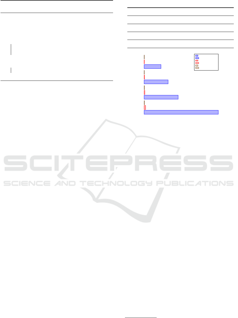
Table 1: Details on the generated datasets.
Trees Σ Arity T D size Gb
D1 500 [2, 12] [1, 5] [10,20] 1.5
D2 800 [2, 12] [1, 5] [10, 50] 2.5
D3 3000 [2, 12] [2, 5] [10, 50] 4.4
D4 4500 [2, 12] [2, 5] [10, 50] 7
D4
D3
D2
D1
97.2
139.7
197
431
0.87
1.96
3.75
8.67
0.81
1.3
1.84
2.63
Sequential
Hadoop
Spark
Figure 3: Performances of Parallel algorithm vs the Sequen-
tial one in terms of running time (minutes).
their average tree size in three classes (small: less than
2GB, medium: less than 2.5GB, and large: more than
4GB). Table 1 illustrates more details on the gener-
ated datasets.
Both sequential and parallel algorithms are imple-
mented in Java 11. All experiments were performed
on a server equipped with an Intel(R) Xeon(R) Sil-
ver 4216 CPU (2.10GHz) processor with 32 cores and
128GB of RAM running Linux.
Sequential and parallel codes in addition to the
generated datasets are available on Github.
In this study, we have established a fixed cluster
architecture, utilizing Docker containers for conduct-
ing all tests. Our cluster comprises one container des-
ignated as the Master, and five containers serving as
Slaves. It is important to note that this choice of clus-
ter configuration was made arbitrarily for the purpose
of this research. The Hadoop
1
V 3.3.0 is installed as
MapReduce implementation platform on our cluster
and Spark
2
V 3.4.1 to serve as the infrastructure for
running Spark.
4.2 Results
Figure 3 reports the performances of our parallel Sub-
Tree Kernel computation versus the sequential al-
gorithm in terms of running time on the generated
datasets. Let us mention that the sequential time is
obtained on one node (container) of our cluster.
1
https://hadoop.apache.org/
2
https://spark.apache.org/
Parallel Tree Kernel Computation
335

It is obvious to observe that our parallel computa-
tion is significantly faster compared to the sequential
version across all dataset instances. Furthermore, our
analysis reveals that the average absolute acceleration
achieved using MapReduce is 50.8 times (Table 2),
and the absolute acceleration obtained through Spark
is 94.3 times (Table 3). This substantial acceleration
is notable, which reflects the effectiveness of our par-
allel computation approach.
Table 2: Acceleration of Parallel SubTree Kernel computa-
tion on different datasets using MapReduce.
D1 D2 D3 D4 Average
A
abs
57.2 62.9 42.6 40.7 50.8
Table 3: Acceleration of Parallel SubTree Kernel computa-
tion on different datasets using Spark.
D1 D2 D3 D4 Average
A
abs
61.4 95 86.8 134.3 94.3
5 CONCLUSION
The prefix tree automaton constitutes a common base
for the computation of different tree kernels: SubTree,
RootedTree, and SubSequenceTree kernels (Ouali-
Sebti, 2015). In this paper, we have shown a paral-
lel Algorithm that efficiently compute this common
structure (RWTA automaton) and we have used it for
the computation of the SubTree Kernel using MapRe-
duce and Spark frameworks.
Our parallel implementation of the SubTree kernel
computation has been tested on synthetic datasets
with different parameters. The results showed that our
parallel computation is by far more speed than the se-
quential version for all instances of datasets. Despite
that this work has shown the efficiency of the paral-
lel implementation compared to the sequential algo-
rithms, three main future works are envisaged. Firstly,
we have to devise some algorithms that generalise
the computation of others kernels such RootedTree,
and SubSequenceTree . . . . Some of them will deploy
tree automata intersection in addition to the associ-
ated weights computation. In fact, while the subtree
kernel is a simple summation of weights, the SubSe-
quenceTree needs more investigation on the weight
computations using the resulted RWTAs intersection.
Secondly, more large datasets have to be generated
and tested to confirm the output-sensitive results of
our solutions. Finally, one can investigate different
cluster architectures in order to give more insights and
recommendations on the cluster’ parameters tuning.
REFERENCES
Alian, M. and Awajan, A. (2023). Syntactic-semantic simi-
larity based on dependency tree kernel. Arabian Jour-
nal for Science and Engineering, pages 1–12.
Chali, Y. and Hasan, S. A. (2015). Towards topic-
to-question generation. Computational Linguistics,
41(1):1–20.
Collins, M. and Duffy, N. (2001). Convolution kernels for
natural language. In Dietterich, T., Becker, S., and
Ghahramani, Z., editors, Advances in Neural Informa-
tion Processing Systems, volume 14. MIT Press.
Collins, M. and Duffy, N. P. (2002). New ranking algo-
rithms for parsing and tagging: Kernels over discrete
structures, and the voted perceptron. In Annual Meet-
ing of the Association for Computational Linguistics.
Dayalan, M. (2004). Mapreduce: simplified data processing
on large clusters. In CACM.
´
Esik, Z. and Kuich, W. (2002). Formal tree series. BRICS
Report Series, (21).
Fu, D., Xu, Y., Yu, H., and Yang, B. (2017). Wastk: An
weighted abstract syntax tree kernel method for source
code plagiarism detection. Scientific Programming,
2017.
Gordon, M. and Ross-Murphy, S. B. (1975). The structure
and properties of molecular trees and networks. Pure
and Applied Chemistry, 43(1-2):1–26.
Haussler, D. et al. (1999). Convolution kernels on discrete
structures. Technical report, Citeseer.
L. Mignot, F. O. and Ziadi, D. (2023). New linear-time al-
gorithm for subtree kernel computation based on root-
weighted tree automata.
Maneth, S., Mihaylov, N., and Sakr, S. (2008). Xml tree
structure compression. In 2008 19th International
Workshop on Database and Expert Systems Applica-
tions, pages 243–247.
Mignot, L., Sebti, N. O., and Ziadi, D. (2015). Root-
weighted tree automata and their applications to tree
kernels. CoRR, abs/1501.03895.
Nasar, Z., Jaffry, S. W., and Malik, M. K. (2021). Named
entity recognition and relation extraction: State-of-
the-art. ACM Comput. Surv., 54(1).
Ouali-Sebti, N. (2015). Noyaux rationnels et automates
d’arbres.
Shatnawi, M. and Belkhouche, B. (2012). Parse trees of
arabic sentences using the natural language toolkit.
Thom, J. D. (2018). Combining tree kernels and text em-
beddings for plagiarism detection. PhD thesis, Stel-
lenbosch: Stellenbosch University.
Vishwanathan, S. V. N. and Smola, A. (2002). Fast kernels
for string and tree matching. In NIPS.
Warikoo, N., Chang, Y.-C., and Hsu, W.-L. (2018). Lptk:
a linguistic pattern-aware dependency tree kernel ap-
proach for the biocreative vi chemprot task. Database,
2018.
ICPRAM 2024 - 13th International Conference on Pattern Recognition Applications and Methods
336