
Combining Total Variation and Nonlocal Variational Models for
Low-Light Image Enhancement
Daniel Torres
a
, Catalina Sbert
b
and Joan Duran
c
Department of Mathematics and Computer Science & IAC3, University of the Balearic Islands,
Cra. de Valldemossa, km. 7.5, E-07122 Palma, Illes Balears, Spain
Keywords:
Low-Light Image Enhancement, Illumination Estimation, Reflectance Estimation, Retinex, Variational
Method, Total Variation, Nonlocal Regularization.
Abstract:
Images captured under low-light conditions impose significant limitations on the performance of computer
vision applications. Therefore, improving their quality by discounting the effects of the illumination is crucial.
In this paper, we present a low-light image enhancement method based on the Retinex theory. Our approach
estimates illumination and reflectance in two steps. First, the illumination is obtained as the minimizer of an
energy functional involving total variation regularization, which favours piecewise smooth solutions. Next,
the reflectance component is computed as the minimizer of an energy functional involving contrast-invariant
nonlocal regularization and a fidelity term preserving the largest gradients of the input image.
1 INTRODUCTION
Enhancing images captured under low-light condi-
tions is crucial for many applications in computer vi-
sion. Various strategies have been proposed to tackle
this problem (Wang et al., 2020), broadly classified
into histogram equalization (Thepade et al., 2021;
Paul et al., 2022), Retinex-based methods, fusion ap-
proaches (Fu et al., 2016a; Buades et al., 2020), and
deep-learning techniques.
The Retinex theory (Land and McCann, 1971),
which aims to explain and simulate how the human
visual system perceives color independently of global
illumination changes, has been an important basis for
addressing low-light image enhancement. One of the
most used models assumes that the observed image L
is the product of the illumination T , which depicts the
light intensity on the objects, and the reflectance R,
which represents their physical characteristics:
L = R ◦T, (1)
where ◦ denotes pixel-wise multiplication. The illu-
mination map is assumed to be smooth, while the re-
flectance component contains fine details and texture
(Ng and Wang, 2011; Li et al., 2018).
a
https://orcid.org/0009-0000-5829-8557
b
https://orcid.org/0000-0003-1219-4474
c
https://orcid.org/0000-0003-0043-1663
Decomposing an image into illumination and re-
flectance is mathematically ill-posed. To address this
issue, patch-based (Land and McCann, 1971), par-
tial differential equations (Morel et al., 2010), cen-
ter/surround (Jobson et al., 1996) and variational
(Kimmel et al., 2001; Ng and Wang, 2011; Ma and
Osher, 2012; Fu et al., 2016b; Guo et al., 2017; Gu
et al., 2019) methods have been proposed.
Recently, the growing popularity of deep learning
has lead to an increase in enhancement methods (Wei
et al., 2018; Lv et al., 2021). However, the structure
of these architectures is often non-intuitive, and their
training and testing require high computational costs.
In this paper, we present a low-light image en-
hancement method taking into account the decompo-
sition model given in (1). We propose to estimate illu-
mination and reflectance separately. In the first step,
the illumination component is obtained as the mini-
mizer of an energy functional involving total varia-
tion (TV) regularization (Rudin et al., 1992), which
favours piecewise smooth solutions. We assume that
the channels of color images share the same illumina-
tion map. In a second step, the reflectance component
is computed as the minimizer of an energy involving
nonlocal regularization, which exploits image self-
similarities, and a fidelity term preserving the large
gradients of the input low-light image. Importantly,
the nonlocal regularization depends on a weight func-
tion that is contrast-invariant.
508
Torres, D., Sbert, C. and Duran, J.
Combining Total Variation and Nonlocal Variational Models for Low-Light Image Enhancement.
DOI: 10.5220/0012386300003660
Paper published under CC license (CC BY-NC-ND 4.0)
In Proceedings of the 19th International Joint Conference on Computer Vision, Imaging and Computer Graphics Theory and Applications (VISIGRAPP 2024) - Volume 3: VISAPP, pages
508-515
ISBN: 978-989-758-679-8; ISSN: 2184-4321
Proceedings Copyright © 2024 by SCITEPRESS – Science and Technology Publications, Lda.

2 RELATED WORK
In the variational framework, the enhanced image is
computed as the minimizer of an energy functional
that comprises data-fidelity and regularization terms.
The latter quantifies the smoothness of the solution
by usually prescribing priors on the gradient of the
illumination or reflectance components.
Kimmel et al. (Kimmel et al., 2001) pioneered
a variational model to estimate the illumination in a
multiscale setting. The illumination is assumed to be
spatially smooth, thus gradient oscillations are penal-
ized through L
2
norm. Ma et al. (Ma and Osher, 2012)
introduced TV to directly compute the reflectance.
On the contrary, Ng et al. (Ng and Wang, 2011) es-
timate illumination and reflectance simultaneously.
One of the most celebrated works is LIME (Guo
et al., 2017). The authors propose a simple TV vari-
ational model to estimate T . Then, the reflectance is
computed as R =
L
T
γ
+ε
, where ε > 0 is a small con-
stant and T
γ
is the γ-corrected illumination. However,
this strategy tends to amplify the noise, especially in
dark regions. To overcome this issue, the authors pro-
pose as enhanced image R ◦T
γ
+ R
d
◦(1 −T
γ
), with
R
d
being the denoised reflectance. Note that any dis-
crepancy in the illumination will impact the result.
Several other variational methods use logarithms
to linearize (1). However, this transformation ampli-
fies errors in gradient terms. In (Fu et al., 2016b),
weights are introduced to address issues arising from
large gradients when either R or T is small.
3 PROPOSED MODELS
In this section, we introduce our low-light image en-
hancement method. We estimate R and T separately
using two different variational models. Let Ω be an
open and bounded domain in R
n
, with n ≥ 2.
3.1 TV Model for Luminance
Based on the classical ROF denoising model (Rudin
et al., 1992), T is obtained as the minimizer of
Z
Ω
|
DT
|
+ λ
Z
Ω
|T (x) −
ˆ
T (x)|
2
dx, (2)
where
R
Ω
|
DT
|
is the TV semi-norm,
λ > 0 is a trade-off parameter, and
ˆ
T is an
initial illumination estimate computed as
ˆ
T (x) =
max
c∈{R,G,B}
L
c
(x). The assumption underlying TV is
that images consist of connected smooth regions (ob-
jects) surrounded by sharp contours. Accordingly, TV
is a good prior for the luminance since it is optimal
Bookcase Clothes rack Plush toy
Figure 1: Pairs of low-light and ground-truth images from
the LOL dataset (Wei et al., 2018) used for the experiments.
to reduce noise and reconstruct the main geometrical
shape.
The energy in (2) is derived from LIME (Guo
et al., 2017). However, we calculate the minimizer
for the exact functional instead of an approximation.
3.2 Nonlocal Model for Reflectance
To estimate the reflectance component, we use non-
local regularization (Gilboa and Osher, 2009; Duran
et al., 2014), which assumes that images are self-
similar, thereby preserving fine details and texture.
3.2.1 Basic Definitions and Notations
Let u = (u
1
,...,u
C
) : Ω →R
C
be a color image, where
C denotes the number of channels. We also consider
nonlocal functions p = (p
1
,. .., p
C
) : Ω ×Ω → R
C
.
Let ω : Ω×Ω →R
≥0
be a weight function, commonly
defined in terms of differences between patches in u.
Definition 3.1. Given u : Ω → R
C
, its nonlocal gra-
dient ∇
ω
u : Ω ×Ω → R
C
is, for each k ∈ {1,...,C},
(∇
ω
u
k
)(x, y) =
p
ω(x,y) (u
k
(y) −u
k
(x)).
Given p : Ω × Ω → R
C
, its nonlocal divergence
div
ω
p : Ω → R
C
is, for each k ∈ {1,...,C},
(div
ω
p
k
)(x)
=
Z
Ω
p
k
(x,y)
p
ω(x,y) − p
k
(y,x)
p
ω(y,x)
dy.
Definition 3.2. The nonlocal vectorial total variation
(NLVTV) of u ∈ L
1
(Ω;R
C
) is defined as
Z
Ω
|D
ω
u| = sup
p∈Y
−
Z
Ω
⟨u(x),(div
ω
p)(x)⟩dx
,
with Y = {p ∈C
∞
c
(Ω×Ω; R
C
) : |p|
NL
(x) ≤1,∀x ∈Ω}
and |p|
NL
(x) =
q
∑
C
k=1
R
Ω
(p
k
(x,y))
2
dy.
3.2.2 Nonlocal Energy Functional
We propose to estimate the reflectance R : Ω → R
C
,
usually C = 3, as the minimizer of the functional
Combining Total Variation and Nonlocal Variational Models for Low-Light Image Enhancement
509
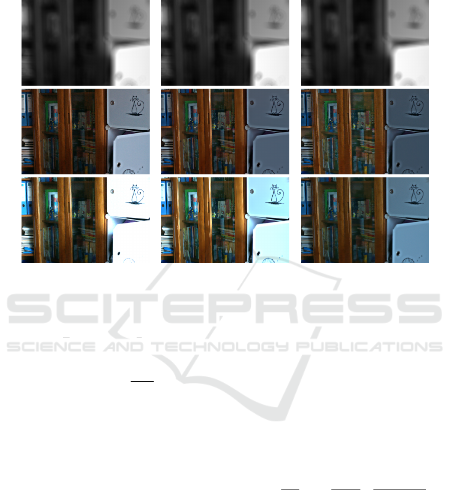
λ = 0.005 λ = 0.05 λ = 0.5
Figure 2: Visual impact of the trade-off parameter λ in (2). Each row contains the illumination, reflectance and enhanced
image, respectively. We observe a piecewise smooth illumination in all cases. However, the differences are more noticeable
in the reflectances and the enhanced images. Indeed, the smaller λ is, the brighter the result.
β
Z
Ω
|D
ω
R|+
α
2
Z
Ω
|∇R −G|
2
+
1
2
Z
Ω
|R −R
0
|
2
, (3)
where α,β > 0 are trade-off parameters,
R
Ω
|D
ω
R| is
the NLVTV, and R
0
is an initial estimate of the re-
flectance computed as R
0
(x) =
L(x)
T (x)+ε
, with T being
the minimizer of (2) and ε > 0 a small constant. The
weight function ω will be defined in terms of differ-
ences between patches in L. Therefore, the underlying
assumption behind NLVTV is that images are self-
similar, making it a good prior for the reflectance.
The second term in (3) enforces closeness be-
tween the gradients of the reflectance and those of an
adjusted version of the low-light image, strengthening
the structural information. Following (Li et al., 2018),
we define G =
1 + λ
G
e
−|∇
ˆ
L|/σ
G
◦∇
ˆ
L, with
∇
ˆ
L =
0 if |∇L| < ε
G
,
∇L otherwise,
where σ
G
controls the amplification rate of different
gradients, λ
G
controls the degree of the amplification,
and ε
G
is the threshold that filters small gradients.
3.2.3 Contrast-Invariant Weights
For the function ω : Ω × Ω → R
≥0
involved in
NLVTV, we propose to use bilateral weights that con-
sider both the spatial closeness between points and the
similarity in L : Ω → R
C
. This similarity is computed
by considering a whole patch around each point and
using the Euclidean distance across color channels:
d (L(x), L(y))
=
Z
Ω
|
(L(x + z) −µ(x)) −(L(y + z) −µ(y))
|
2
dz,
(4)
where µ(x) denotes the mean value of the patch cen-
tered at x. This allows the distance (4) to be contrast
invariant between the selected patches.
The weights are defined as
ω(x,y) =
1
Γ(x)
exp
−
|x −y|
2
h
2
spt
−
d(L(x),L(y))
h
2
sim
!
(5)
where h
spt
,h
sim
> 0 are filtering parameters that con-
trol how fast the weights decay with increasing spa-
tial distance or dissimilarity between patches, respec-
tively, and Γ(x) is the normalization factor. Note that
0 < ω(x,y) ≤1 and
R
Ω
ω(x,y) dy = 1, but Γ(x) breaks
down the symmetry of ω. The average between very
similar regions preserves the integrity of the image
but reduces small oscillations, which contain noise.
For computational purposes, NLVTV is limited to
interact only between points at a certain distance. Let
VISAPP 2024 - 19th International Conference on Computer Vision Theory and Applications
510
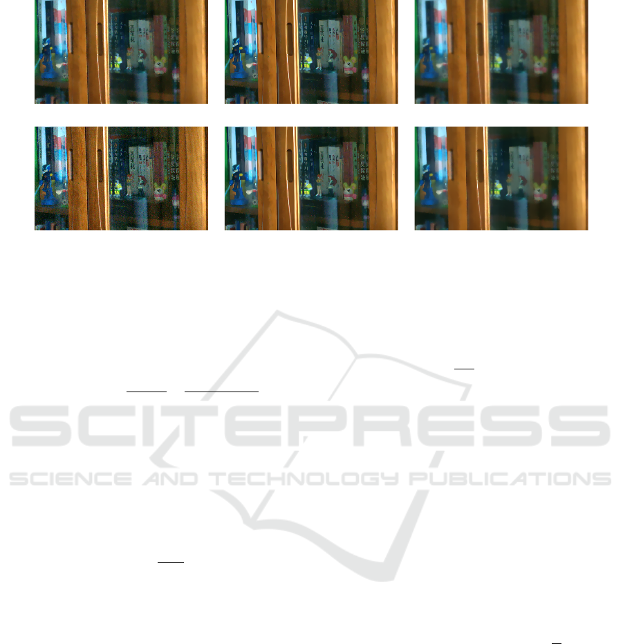
α = 0.0001, β = 0.5 α = 0.01, β = 0.5 α = 1, β = 0.5
α = 0.01, β = 0.05 α = 0.01, β = 0.5 α = 0.01, β = 1
Figure 3: Visual impact of the trade-off parameters α and β in (3) on the final enhanced image. Larger values of α or β result
in an over-smoothed image, as can be appreciated in the third column. On the other hand, when the role of the regularization
term is less relevant, as it is the case for β = 0.05, the noise is enhanced in the final result.
N (x) denote a neighbourhood around x ∈ Ω. Then,
ω(x,y) is defined as in (5) if y ∈ N (x), and zero oth-
erwise. The normalization factor is finally given by
Γ(x) =
Z
N (x)
exp
−
|x −y|
2
h
2
spt
−
d (L(x), L(y))
h
2
sim
!
dy.
3.3 Enhanced Image
Once we obtain the illumination and the reflectance,
we need to adjust the lighting by applying a gamma
correction with parameter γ > 0 to T , helping us ad-
dress the over-saturation problem. This transforma-
tion involves the following operation at each pixel:
T
′
(x) = S
T (x)
S
γ
, (6)
where S is a constant typically set to 1 to ensure that
the inputs and outputs are within the same range. Fi-
nally, the enhanced image is computed as L
′
= R ◦T
′
.
4 PRIMAL-DUAL
OPTIMIZATION
In the discrete setting, L,R ∈ R
N×C
and T ∈ R
N
,
where N is the number of pixels and C is the num-
ber of channels. Both ∇T ∈ R
N×2
and ∇R ∈ R
N×C×2
are computed via forward differences and Neumann
boundary conditions, and denoted for each pixel i
and channel k by (∇T)
i
= ((∇T )
i,1
,(∇T )
i,2
) and
(∇R)
i,k
= ((∇R)
i,k,1
,(∇R)
i,k,2
), respectively.
Let M be the size of the neighborhood around
each pixel where the weights of the NLVTV regu-
larization term are nonzero. The nonlocal gradient
∇
ω
R ∈R
N×C×M
, denoted for each pixel i and channel
k by (∇
ω
R)
i,k
= ((∇
ω
R)
i,k,1
,. ..,(∇
ω
R)
i,k,M
), is de-
fined as (∇
ω
R)
i,k, j
=
√
ω
i, j
R
j,k
−R
i,k
, where {ω
i, j
}
contains the discretization of the weights (5). In prac-
tice, the weight of the reference pixel is set to the
maximum of the weights in the neihbourhood, i.e.,
ω
i,i
= max
1≤j≤M
ω
i, j
. This setting avoids the exces-
sive weighting of the reference pixel.
Both minimization problems (2) and (3) are con-
vex but non-smooth. To find a global optimal so-
lution, we use the first-order primal-dual algorithm
introduced in (Chambolle and Pock, 2011). To do
so, we rewrite each problem in a saddle-point for-
mulation by introducing dual variables. The algo-
rithm consists of alternating a gradient ascent in the
dual variable, a gradient descent in the primal variable
and an over-relaxation for convergence purposes. The
gradient steps are given in terms of the proximity op-
erator, which is defined for any proper convex func-
tion ϕ as prox
τ
ϕ(x) = arg min
y
{ϕ(y) +
1
2τ
∥x −y∥
2
2
}.
The efficiency of the algorithm is based on the as-
sumption that proximity operators have closed-form
representations or can be efficiently solved. For all
details on convex analysis omitted in this section, we
refer to (Chambolle and Pock, 2016).
4.1 Estimation of the Illumination
The discrete variational model related to (2) is
min
T ∈R
N
∥∇T ∥
1
+ λ∥T −
ˆ
T ∥
2
2
, (7)
Combining Total Variation and Nonlocal Variational Models for Low-Light Image Enhancement
511

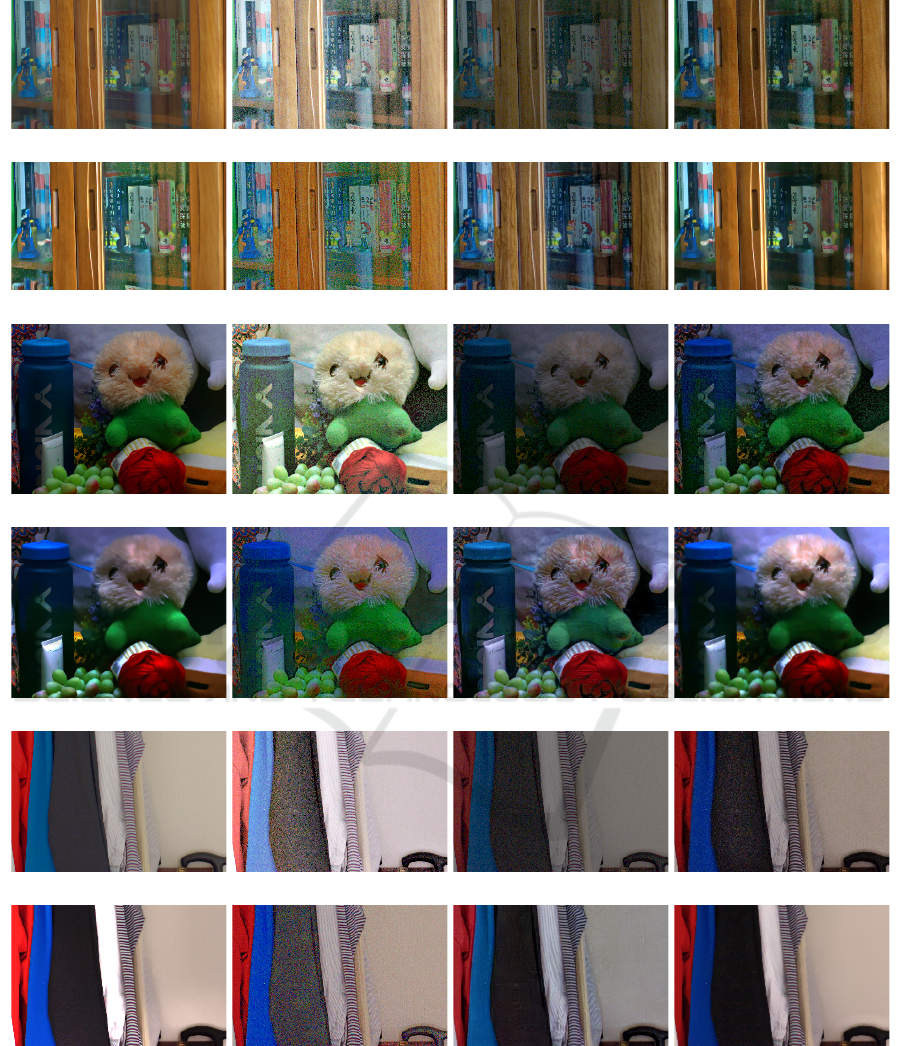
γ = 0.25 γ = 0.4 γ = 0.55
Figure 4: Study of the effect of the gamma correction (6) with parameter γ. In the first row, we display the γ-corrected
illuminations and the second row contains the resulting enhanced images. We observe that an excessive gamma correction
(γ = 0.25) leads to a saturated image, while a less significant transformation (γ = 0.55) results in an overly dark image.
where ∥∇T ∥
1
=
∑
N
i=1
|(∇T )
i
|. The saddle-point for-
mulation of (7) is given by
min
T ∈R
N
max
p∈P
⟨∇T, p⟩−δ
P
(p) + λ∥T −
˜
T ∥
2
2
,
where P = {p ∈ R
N×2
: |p
i,:
| ≤ 1,∀i} and δ
P
is the
indicator function of P .
Therefore, T is computed through the following
primal-dual iterates:
p
n+1
i, j
=
p
n
i, j
+ σ(∇T
n
)
i, j
max
1,|p
n
i
+ σ(∇T
n
)
i
|
,
T
n+1
=
T
n
+ τ divp
n+1
+ τλ
ˆ
T
1 + τλ
,
T
n+1
= 2T
n+1
−T
n
.
4.2 Estimation of the Reflectance
The discretization of the variational model (3) is
β∥∇
ω
R∥
1
+
α
2
∥∇R −G∥
2
2
+
1
2
∥R −R
0
∥
2
2
, (8)
where ∥∇
ω
R∥
1
=
∑
N
i=1
q
∑
C
k=1
|(∇
ω
R)
i,k
|
2
and ∥·∥
2
applies across channel and pixel dimensions.
The NLVTV term is treated analogously to the
TV case. We also need to dualize the α-term since
its proximity operator has no closed-form. By tak-
ing into account that
α
2
∥x∥
2
2
= sup
y
⟨x,y⟩−
1
2α
∥y∥
2
2
, the
saddle-point formulation of (8) is
min
R∈R
N×C
max
p∈R
N×C×2
,q∈Q
⟨∇R, p⟩+ ⟨∇
ω
R,q⟩
−
1
2α
∥p −G∥
2
2
−δ
Q
(q) +
1
2
∥R −R
0
∥
2
2
,
with Q = {q ∈ R
N×C×M
:
∑
C
k=1
∑
M
j=1
q
2
i,k, j
≤ β
2
,∀i}.
Therefore, R is computed through the following
primal-dual iterates:
p
n+1
=
α
p
n
+ σ∇R
n
+ σG
α + σ
,
q
n+1
i,k, j
=
β
q
n
i,k, j
+ σ(∇
ω
R
n
)
i,k, j
max
β,|q
n
i
+ σ(∇
ω
R
n
)
i
|
,
R
n+1
=
R
n
+ τdivp + τdiv
ω
q + τR
0
1 + τ
,
R
n+1
i
= 2R
n+1
i
−R
n
i
.
5 ANALYSIS AND EXPERIMENTS
In this section, we analyze the performance of the pro-
posed method for low-light image enhancement. Fig-
ure 1 displays the pairs of low-light and ground-truth
images from the LOL dataset (Wei et al., 2018) used
in the experiments. We have also used Lamp from
(Guo et al., 2017), a natural low-light image.
5.1 Ablation Study
Figure 2 illustrates the impact of the trade-off param-
eter λ in the variational model (2). We observe that a
piecewise smooth illumination is obtained in all cases.
The slight variation in the illumination is amplified
in the reflectance maps and the enhanced images, re-
sulting in darker or brighter images, depending on
whether more or less weight is given to the fidelity
term compared to the regularization term.
VISAPP 2024 - 19th International Conference on Computer Vision Theory and Applications
512
Bookcase MSR Kimmel et al. SRIE
LIME RetinexNet AGLLNet Ours
Plush toy MSR Kimmel et al. SRIE
LIME RetinexNet AGLLNet Ours
Clothes rack MSR Kimmel et al. SRIE
LIME RetinexNet AGLLNet Ours
Figure 5: Comparison between state-of-the-art techniques and our method on dataset in Figure 1. We observe that MSR, SRIE
and RetinexNet are not robust to noise and exhibit color issues in all experiments. The method by Kimmel et al. is not able
to correctly remove the effect of the illumination, while LIME produces oversaturated results. AGLLNet produces greyish
images and introduces color artifacts as seen for instance in the blue bottle and the red ball of yarn. Our method provides the
best compromise between discounting the illumination effect, avoiding the amplification of noise, and preserving the color
and geometry structure of the scene.
Combining Total Variation and Nonlocal Variational Models for Low-Light Image Enhancement
513
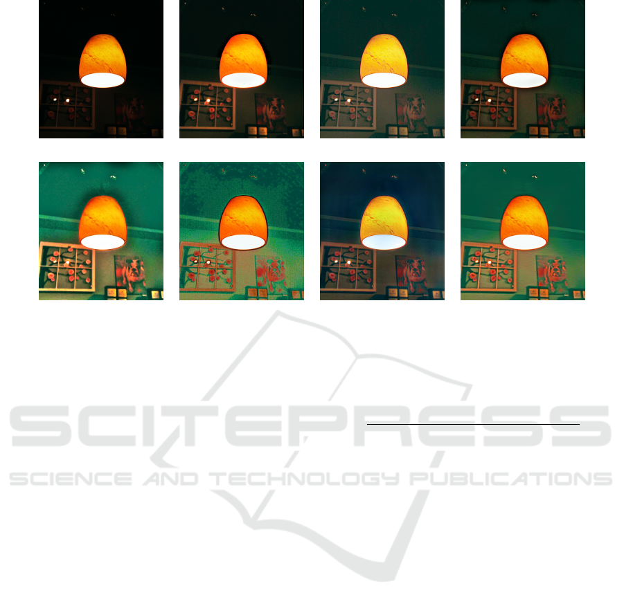
Lamp MSR Kimmel et al. SRIE
LIME RetinexNet AGLLNet Ours
Figure 6: Comparison between state-of-the-art methods and our proposal on a natural low-light image. We observe that only
LIME, RetinexNet and our method are able to remove the effect of the illumination. However, LIME and RetinexNet are
affected by noise and also produce enhanced images with artifacts, like the halo surrounding the lamp.
In Figure 3, we discuss about the influence of the
trade-off parameters α and β in (3) on the enhanced
image produced by the proposed method. We observe
that larger values of α or β result in an over-smoothed
image. On the other hand, when the role of the reg-
ularization term is less relevant, as it is the case for
β = 0.05, the noise is amplified.
Gamma correction is an essential tool for adjust-
ing the lighting, as shown in Figure 4. Indeed, we ob-
serve how varying γ significantly affects the final im-
age: an excessive gamma correction (γ = 0.25) leads
to a saturated image, while a less significant transfor-
mation (γ = 0.55) results in an overly dark image.
5.2 Comparison with the State of the
Art
We compare our method with Multiscale Retinex
(MSR) (Jobson et al., 1997), Kimmel et al. (Kim-
mel et al., 2001), SRIE (Fu et al., 2016b), LIME
(Guo et al., 2017) and the deep learning techniques
RetinexNet (Wei et al., 2018) and AGLLNet (Lv
et al., 2021). Kimmel et al. and LIME have been im-
plemented by ourselves, while SRIE is sourced from
(Ying et al., 2017) and MSR from (Petro et al., 2014).
The trained networks of RetinexNet and AGLLNet
are provided by the authors on their webpages. The
most suitable parameters for state-of-the-art and our
method have been chosen based on visual evaluation.
Table 1: Quantitative evaluation on results in Figure 5.
PSNR ↑ SSIM ↑
MSR 12.41 0.7229
Kimmel et al. 14.27 0.8287
SRIE 17.27 0.8483
LIME 18.09 0.8592
RetinexNet 17.56 0.7819
AGLLNet 16.82 0.8661
Ours 20.08 0.8868
Figure 5 displays a comparison among all meth-
ods on Bookcase, Clothes rack and Plush toy. We
observe that MSR, SRIE and RetinexNet are not ro-
bust to noise and exhibit color issues in all cases. The
method by Kimmel et al. is not able to correctly re-
move the effect of the illumination, while LIME tends
to oversaturate the scene. AGLLNet produces grey-
ish images, introduces color artifacts, as seen in the
blue bottle and the red ball of yarn in Plush toy, and
modifies the texture of the reference image, as seen in
the wood of Bookcase. Our method provides the best
compromise between discounting the illumination ef-
fect, avoiding the amplification of noise, and preserv-
ing the color and geometry structure of the scene.
We also evaluate the performance of all methods
in terms of PSNR and SSIM. Table 1 displays the av-
erage values on the results in Figure 5. Our method
outperforms the others in terms of both metrics.
An additional analysis has been performed with
the natural low-light image Lamp in Figure 6. Only
VISAPP 2024 - 19th International Conference on Computer Vision Theory and Applications
514

LIME, RetinexNet and our method are able to remove
the effect of the illumination. However, LIME and
RetinexNet are affected by noise and also produce ar-
tifacts, like the halo surrounding the lamp.
6 CONCLUSION
In this paper, we have proposed a low-light image en-
hancement method that estimates illumination and re-
flectance separately using variational models. In par-
ticular, we have introduced a contrast-invariant non-
local regularization term for recovering fine details
in the reflectance component. The experiments have
shown that our method obtains state-of-the-art results
and performs well in terms of noise reduction, color
recovery, geometry and texture preservation.
ACKNOWLEDGEMENTS
This work is part of the MaLiSat project TED2021-
132644B-I00, funded by MCIN/AEI/10.13039/
501100011033/ and by the European Union
NextGenerationEU/PRTR, and also of the Mo-
LaLIP project PID2021-125711OB-I00, financed by
MCIN/AEI/10.13039/501100011033/FEDER, EU.
REFERENCES
Buades, A., Lisani, J.-L., Petro, A. B., and Sbert, C.
(2020). Backlit images enhancement using global tone
mappings and image fusion. IET Image Processing,
14(2):211–219.
Chambolle, A. and Pock, T. (2011). A first-order primal-
dual algorithm for convex problems with applications
to imaging. Journal of Mathematical Imaging and Vi-
sion, 40:120–145.
Chambolle, A. and Pock, T. (2016). An introduction to
continuous optimization for imaging. Acta Numerica,
25:161–319.
Duran, J., Buades, A., Coll, B., and Sbert, C. (2014). A
nonlocal variational model for pansharpening image
fusion. SIAM Journal on Imaging Sciences, 7(2):761–
796.
Fu, X., Zeng, D., Huang, Y., Liao, Y., Ding, X., and Pais-
ley, J. (2016a). A fusion-based enhancing method
for weakly illuminated images. Signal Processing,
129:82–96.
Fu, X., Zeng, D., Huang, Y., Zhang, X., and Ding, X.
(2016b). A weighted variational model for simulta-
neous reflectance and illumination estimation. CVPR,
pages 2782–2790.
Gilboa, G. and Osher, S. (2009). Nonlocal operators with
applications to image processing. Multiscale Model-
ing & Simulation, 7(3):1005–1028.
Gu, Z., Li, F., and Lv, X.-G. (2019). A detail preserving
variational model for image retinex. Applied Mathe-
matical Modelling, 68:643–661.
Guo, X., Yu, L., and Ling, H. (2017). Lime: Low-light
image enhancement via illumination map estimation.
IEEE Transactions on Image Processing, 26(2):982–
993.
Jobson, D., Rahman, Z., and Woodell, G. (1996). Properties
and performance of a center/surround retinex. TIP,
6(3):451–462.
Jobson, D., Rahman, Z., and Woodell, G. (1997). A multi-
scale retinex for bridging the gap between color im-
ages and the human observation of scenes. IEEE
Transactions on Image Processing, 6(7):965–976.
Kimmel, R., Elad, M., Shaked, D., Keshet, R., and Sobel,
I. (2001). A variational framework for retinex. Int. J.
Comput. Vis., 52(1):7–23.
Land, E. H. and McCann, J. J. (1971). Lightness and retinex
theory. Journal of the Optical Society of America,
61(1):1–11.
Li, M., Liu, J., Yang, W., Sun, X., and Guo, Z. (2018).
Structure-revealing low-light image enhancement via
robust retinex model. IEEE Transactions on Image
Processing, pages 2828–2841.
Lv, F., Yu, L., and Lu, F. (2021). Attention guided low-
light image enhancement with a large scale low-light
simulation dataset. International Journal of Computer
Vision, pages 2175—-2193.
Ma, W. and Osher, S. (2012). A tv bregman iterative model
of retinex theory. Inverse Problems and Imaging,
6(4):697–708.
Morel, J. M., Petro, A. B., and Sbert, C. (2010). A pde
formalization of retinex theory. IEEE Transactions on
Image Processing, 19(11):2825–2837.
Ng, M. K. and Wang, W. (2011). A total variation model
for retinex. SIAM J. Imag. Sci., 4(1):345–365.
Paul, A., Bhattacharya, P., and Maity, S. P. (2022). His-
togram modification in adaptive bi-histogram equal-
ization for contrast enhancement on digital images.
Optik, 259:168899.
Petro, A. B., Sbert, C., and Morel, J. M. (2014). Multiscale
retinex. Image Processing On Line, pages 71–88.
Rudin, L. I., Osher, S., and Fatemi, E. (1992). Nonlinear to-
tal variation based noise removal algorithms. Physica
D: Nonlinear Phenomena, 60(1):259–268.
Thepade, S. D., Ople, M., Mahindra, V., Kulye, V., and
Jamdar, S. (2021). Low light image contrast enhance-
ment using blending of histogram equalization based
methods bbhe and bpheme. In 2021 International
Conference on Disruptive Technologies for Multi-
Disciplinary Research and Applications (CENTCON),
volume 1, pages 259–264.
Wang, W., Wu, X., and snd Z. Guo, X. Y. (2020). An
experiment-based review of low-light image enhance-
ment methods. IEEE Access, 8:87884–87917.
Wei, C., Wang, W., Yang, W., and Liu, J. (2018). Deep
retinex decomposition for low-light enhancement.
BMVC.
Ying, Z., Li, G., and Gao, W. (2017). A bio-inspired multi-
exposure fusion framework for low-light image en-
hancement.
Combining Total Variation and Nonlocal Variational Models for Low-Light Image Enhancement
515
