
Understanding Marker-Based Normalization for FLIM Networks
Leonardo de Melo Joao
1,2 a
, Matheus Abrantes Cerqueira
1 b
, Barbara Caroline Benato
1 c
and Alexandre Xavier Falcao
1 d
1
Institute of Computing, State University of Campinas, Campinas, 13083-872, S
˜
ao Paulo, Brazil
2
LIGM, Univ. Gustave-Eiffel, Marne-la-Val
´
ee, F-77454, France
Keywords:
Marker-Based-Normalization, Flim, Z-Score-Normalization, Object-Detection.
Abstract:
Successful methods for object detection in multiple image domains are based on convolutional networks.
However, such approaches require large annotated image sets for network training. One can build object
detectors by exploring a recent methodology, Feature Learning from Image Markers (FLIM), that considerably
reduces human effort in data annotation. In FLIM, the encoder’s filters are estimated among image patches
extracted from scribbles drawn by the user on discriminative regions of a few representative images. The filters
are meant to create feature maps in which the object is activated or deactivated. This task depends on a z-score
normalization using the scribbles’ statistics, named marker-based normalization (MBN). An adaptive decoder
(point-wise convolution with activation) finds its parameters for each image and outputs a saliency map for
object detection. This encoder-decoder network is trained without backpropagation. This work investigates the
effect of MBN on the network’s results. We detach the scribble sets for filter estimation and MBN, introduce
a bot that draws scribbles with distinct ratios of object-and-background samples, and evaluate the impact of
five different ratios on three datasets through six quantitative metrics and feature projection analysis. The
experiments suggest that scribble detachment and MBN with object oversampling are beneficial.
1 INTRODUCTION
Object detection has been widely studied in com-
puter vision with several applications (Kaur and
Singh, 2022). Object detection is commonly used
for estimating (and often classifying) bounding boxes
around objects. Alternatively, Salient Object Detec-
tion (SOD) methods are suitable for single-class tasks
— minimum bounding boxes can be estimated around
the salient objects (Joao et al., 2023). We adopt
this second approach. The best-performing methods
are based on deep neural networks, mostly Convolu-
tional Neural Networks (CNNs) (Zaidi et al., 2022).
However, they require considerable computational re-
sources and human effort in data annotation.
Human effort and computational resources can
be significantly reduced with a recent methodology
named Feature Learning by Image Markers (FLIM)
for training convolutional encoders without backprop-
agation (De Souza and Falc
˜
ao, 2020). In FLIM, the
a
https://orcid.org/0000-0003-4625-7840
b
https://orcid.org/0000-0003-3655-3435
c
https://orcid.org/0000-0003-0806-3607
d
https://orcid.org/0000-0002-2914-5380
user draws scribbles on discriminative regions of very
few (e.g., 5) representative images. The encoder’s fil-
ters of the first convolutional layer are estimated from
patches centered at scribble pixels. The process re-
peats for each subsequent layer by mapping the scrib-
bles onto the output of the previous one. For a single-
class object detection problem, each filter is meant to
activate the object or background (Figure 1). The suc-
cess of this task depends on a z-score normalization
using the scribbles’ statistics, named marker-based
normalization (MBN). Such foreground and back-
ground activations favor using a single-layer decoder
(point-wise convolution with activation) that adapts
the weights for each image and outputs a saliency map
suitable for object detection. In (Joao et al., 2023), the
authors explore this methodology to create flyweight
encoder-decoder networks for object detection with
competitive results to fully pretrained deep models.
A patch centered at a pixel can be represented by a
vector with the attributes of its pixels. The dot product
between a filter’s weight vector and each image patch
corresponds to the convolution operation. The lower
the angle between filter and patch vectors, the higher
the dot product between them (i.e., the similarity be-
612
Joao, L., Cerqueira, M., Benato, B. and Falcao, A.
Understanding Marker-Based Normalization for FLIM Networks.
DOI: 10.5220/0012385900003660
Paper published under CC license (CC BY-NC-ND 4.0)
In Proceedings of the 19th International Joint Conference on Computer Vision, Imaging and Computer Graphics Theory and Applications (VISIGRAPP 2024) - Volume 2: VISAPP, pages
612-623
ISBN: 978-989-758-679-8; ISSN: 2184-4321
Proceedings Copyright © 2024 by SCITEPRESS – Science and Technology Publications, Lda.

(a) (b) (c)
Figure 1: Foreground and background filter activations on
a parasite egg image. (a) Original Image; (b-c) Foreground
and Background activations. An yellow arrow points the
object of interest.
tween their visual patterns). The patches extracted
from the scribbles may form distinct groups in a patch
feature space. MBN aims to centralize the groups and
correct distortions among attributes. In FLIM, each
group center generates one filter. For foreground and
background activations, MBN should increase the an-
gle between such groups as much as possible.
Figure 2.a illustrates four groups of patches such
that filters from groups green and red generate simul-
taneous and redundant activation maps. MBN aims to
create group distributions, as depicted in Figure 2.b,
which presents higher angular distances among the
groups. Estimating the z-score normalization param-
eters from the scribbles’ statistics is crucial to achiev-
ing that aim due to the natural imbalance between
the numbers of foreground and background patches
within an image. Z-score normalization using statis-
tics from all pixels would likely create a group distri-
bution, as depicted in Figure 2.c, where the less dense
classes’ statistics are not considered.
Understanding the impact of drawing more or
fewer markers in the foreground or background for
MBN can guide users’ actions when building the net-
work. However, FLIM uses the same scribble set for
filter estimation and MBN. In this work, we investi-
gate the impact of MBN on the network results for
object detection by detaching the parts of the scrib-
bles used for each operation. No studies so far have
addressed the role of MBN in the network construc-
tion process.
For this study, we developed a marker bot to draw
disks in the foreground and background parts and ex-
tend them into scribbles inside each part. Scribble
drawing is a controlled process such that we can gen-
erate a distinct ratio between object and background
patches. We evaluate the impact of MBN using three
datasets, five different ratios – balanced (1:1) and im-
balanced (1:10, 1:50) for both background and fore-
ground –, and six metrics of object detection with vi-
sual analysis of feature space projections (Zeiler et al.,
2014; Rauber et al., 2017). Additionally, we compare
the results with the traditional FLIM in which filter
estimation and MBN use the same scribble set.
The contributions of this paper are four-fold: (i)
understanding the isolated impact of MBN within
FLIM networks using metrics and visualization; (ii)
understanding the impact of different foreground-
and-background ratios when learning the normaliza-
tion parameters for FLIM networks; (iii) a mathemat-
ical interpretation of the role of (marker-based) nor-
malization in creating feature spaces suitable for con-
volution; and (iv) a marker bot for drawing scribbles
based on ground truth masks for training FLIM net-
works.
2 RELATED WORK
The literature has a range of approaches to normal-
ization that vary in complexity and robustness to out-
liers, such as min-max, which is simpler but signifi-
cantly impacted by outliers, and z-score, which uses
the mean and deviation as measures of location and
scale. Tanh-estimators are less sensitive to outliers
but require parameter configuration(Jain et al., 2005).
There is no consensus on a single method (Omar et al.,
2022), but z-score normalization is very relevant as it
is one of the most common normalization methods.
Z-score normalization assumes the data to be nor-
mally distributed (Jain et al., 2005), which often is
not the case in images with a large imbalance of fore-
ground and background pixels (as discussed in Fig-
ure 2). To circumvent that problem, MBN was pro-
posed and user-drawn scribbles were used to under-
sample the data for learning the normalization param-
eters (De Souza and Falc
˜
ao, 2020).
MBN was used in several works together
with FLIM CNNs, and is suitable for classifica-
tion (De Souza and Falc
˜
ao, 2020), object detec-
tion (Joao et al., 2023), and segmentation tasks (Sousa
et al., 2021; Cerqueira et al., 2023) in multiple image
domains. However, none of these methods studied
the impact of different scribble sets for the normaliza-
tion parameters. In this work, we propose to analyze
that impact by looking at feature space projections
and the object detection result of an encoder-decoder
network.
3 BACKGROUND
In this section, we provide the definitions required
for our proposal and discussions (Section 3.1), an
overview of how to train FLIM networks for object
detection (Section 3.2), a formalization of the Marker-
based normalization (Section 3.3), and some math-
ematical interpretations of convolutions, dot prod-
uct and the normalization impact for creating feature
Understanding Marker-Based Normalization for FLIM Networks
613
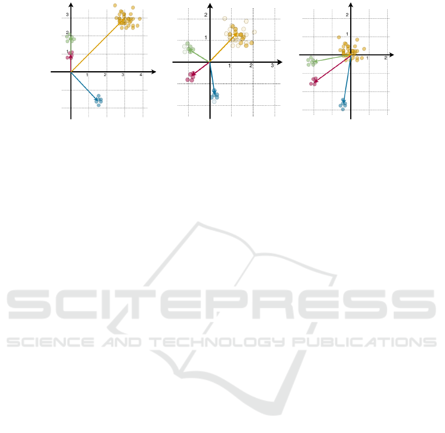
(a) (b) (c)
Figure 2: Impacts of normalization: (a) original space; (b) desired normalization; (c) z-score normalization of entire data.
spaces suitable for these operations (Section 3.4).
3.1 Definitions
Images, Adjacency Relations, and Image Patches:
Let an image be defined by X ∈ R
h×w×c
where h × w
are its dimension with c number of channels. Con-
sidering i ∈ {1, h}, j ∈ {1,w}, a pixel at position (i, j)
can be seen as its feature vector x
i j
∈ R
c
, with its b-th
channel (feature) value being x
i jb
∈ R,b ∈ {1, c}.
Let u ∈ {1,h},v ∈ {1,w}, and p = (i, j),q = (u,v)
be the coordinates of image pixels. An adjacency rela-
tion A can be defined as a binary translation-invariant
relation between pixels (p,q). In this work, two adja-
cency relations are used. For annotating the scribbles,
we use a circular relation A
c
with radius ρ ≥ 0, which
is defined by A
c
: {(p,q)| ∥q − p∥ ≤ ρ}.
For the convolution operations and kernel estima-
tions, we use image patches contained within a square
relation A
s
of size a ≥ 0, defined by A
s
: {(p,q)| |x
q
−
x
p
| ≤ a,|y
q
− y
p
| ≤ a}.
In any case, A(p) is a set of pixels q ∈ Z
2
adjacent
to p. Zero-padding is done so all image pixels to have
the same size for their adjacency relations.
Lastly, an image patch p
p
∈ R
a×a×c
, is a sub-
image with the c features of all a × a pixels in A
s
(p).
Filters and Convolutions. A kernel (or filter) k ∈
R
a×a×c
is a matrix with the same shape as a patch.
Within a CNN, the convolution of an image with a
filter can be described as Y = X ⋆ k. Assuming zero
padding, Y ∈ R
h×w×1
and y
i j
∈ Y.
Let p
p
and
˜
k be represented as flattened vectors
˜
p
p
,
˜
k ∈ R
d
, such that d = a · a · c. The value of y
p
can
be computed by the dot product between the kernel
and patch vectors:
y
i j
= ⟨
˜
p
p
,
˜
k⟩ (1)
with ⟨
˜
p
p
,
˜
k⟩ = ∥
˜
p
p
∥∥
˜
k∥cos θ,
where θ is the angle between both vectors.
3.2 FLIM Networks
FLIM is a methodology to create feature extractors
(encoders) to compose convolutional blocks of CNNs.
In FLIM, kernels are estimated from image patches
centered on marked pixels, which are also used to
learn the normalization parameters. The FLIM en-
coders can be combined with different decoders to
provide successful image classification, segmenta-
tion, and object detection solutions. In this section,
we first present the steps for training a FLIM encoder
(Section 3.2.1) and how we can combine it with an
Adaptive Decoder to propose a solution for object de-
tection tasks (Section 3.2.2).
3.2.1 Encoder Learning
FLIM has been described to contain six steps (Joao
et al., 2023):
1. Training Image Selection - For this work, we fol-
low the same strategy as (Joao et al., 2023) and
manually selected a small number of representa-
tive images (1% of the dataset) such that the train-
ing set contains examples of the most visually dis-
tinguishing characteristics among the object class.
2. Marker Drawing - Markers have to be drawn in
the training images. We use the proposed marker-
bot (Section 4.1).
3. Data Preparation - Marker-based normalization
is applied, and the markers are scaled onto the re-
quired image dimension for the layer. This is the
step we are investigating further in this work.
4. Kernel Estimation - Given the training images, a
pre-defined architecture, and image markers, the
convolutional kernels are extracted, respecting the
sizes and numbers defined in the architecture. For
learning the kernels, given an image marker, we
cluster all its marker patches (patches centered on
its pixels) using k-means and take the centers of
VISAPP 2024 - 19th International Conference on Computer Vision Theory and Applications
614

each of the k
m
clusters found as a kernel. Then,
the total number of kernels is reduced using an-
other K-means to fit the required number of filters
in the defined architecture for a given layer.
5. Block Execution - Every image goes through the
transformations within the learned convolutional
block, and the new image features are extracted.
These operations are usually convolution, acti-
vation — commonly the Rectified Linear Unit
(ReLU) (Nair and Hinton, 2010) —, and pooling.
6. Kernel Selection - One may select kernels to re-
duce redundancy, simplifying the network. We do
not explore kernel selection in this work.
After each convolutional block is learned, steps 3-
6 are repeated until the desired network architecture is
achieved, with the previous output being used as the
input for learning the kernels of the next block.
3.2.2 FLIM CNN and Adaptive Decoder
Recently, an unsupervised and adaptive decoder (Joao
et al., 2023) was proposed for creating flyweight
(tiny) CNNs, allowing the creation of fully connected
networks for object detection without the need of
backpropagation.
The adaptive decoders proposed so far are sim-
ply one-layer point-wise convolutions followed by a
ReLU, where the kernel weights are estimated on
the fly according to the input image and an adap-
tation function. Point-wise convolution can be un-
derstood as a weighted sum of all image channels
of the input image. Let A ∈ R
h
′
×w
′
×m
be the out-
put of an encoder’s layer, where h
′
,w
′
are the im-
age image’s height and width after pooling, and α =
[α
1
,α
2
,...,α
m
] ∈ R
m
be the convolutional weights,
such that α
b
∈ [−1,1], and b = 1, 2, ... ,m. The de-
coder is than simply S = ReLU (⟨A,α⟩).
As mentioned, the decoder weights are estimated
by an adaptation function, which is a heuristic based
on prior information about the image domain. For the
target problems, the background is often larger and
somewhat homogeneous, so the adaptation function
defines a kernel to be positive if it has a low mean ac-
tivation value. Let F : α
b
→ {−α, 0,α} be the adap-
tation function, such that:
The literature has a range of approaches to nor-
malization that vary in complexity and robustness to
outliers, such as min-max, which is simpler but signif-
icantly impacted by outliers, and z-score, which uses
the mean and deviation as measures of location and
scale. Tanh-estimators are less sensitive to outliers
but require parameter configuration(Jain et al., 2005).
There is no consensus on a single method (Omar et al.,
2022), but z-score normalization is very relevant as it
is one of the most common normalization methods.
F(A,b) =
+α, if µ
A
b
≤ τ
A
b
+ σ
µ
−α, if µ
A
b
≥ τ
A
b
− σ
µ
0, otherwise.
where τ
A
b
is the Otsu threshold computed for all the
means, ¯µ =
1
m
∑
m
b=1
µ
A
b
and σ
µ
=
1
m
∑
m
b=1
(µ
A
b
− ¯µ)
2
.
By assuming the background and foreground mean
activations to be split between two densities, the Otsu
is used here to find the separation between them.
The decoder outputs a saliency map that, for the
purpose of object detection, can be thresholded us-
ing the Otsu method so that minimum bounding boxes
can be set around the binary connected components.
Combining a FLIM encoder with an unsupervised
adaptation encoder provides a weak supervised ap-
proach for object detection, where the only annota-
tions required are the scribbles from a few training
images.
3.3 Marker-Based Normalization
When learning the Z-score normalization parameters,
FLIM uses the estimated markers to undersample the
data. That operation is called Marker-based Normal-
ization (MBN).. Let X be the set of training images
(the ones containing markers), where an image is de-
noted by X ∈ X , and its marker set by M (X). Also,
let M be the set of all markers, such that
S
X∈X
M (X).
An image X can be normalized into
ˆ
X ∈ R
h×w×m
, by
the following equation:
ˆx
i jb
=
x
i jb
− µ
b
σ
b
+ ε
, (2)
where µ
b
=
1
|M |
∑
∀x
i jb
∈M (X)
x
i jb
, is the mean of the
marker features, σ
2
b
=
1
|M |
∑
∀x
i jb
∈M (X)
x
i jb
− µ
b
2
is
their standard deviation, and ε > 0 is a small constant.
3.4 Mathematical Interpretations
Starting from the convolution operation, as discussed
in (Joao et al., 2023), the dot-product (in Equation 1)
can be interpreted geometrically as a projection of
˜
p
i j
into a hyperplane h positioned at the origin of R
d
that
is perpendicular to
˜
k (Figure 3). This projection can
be seen as a similarity measure scaled by the vectors’
magnitudes. However, it is essentially a signed an-
gular (cosine) distance, where the sign depends on
which side of the hyperplane
˜
p
i j
is.
Understanding Marker-Based Normalization for FLIM Networks
615

By considering convolution as a similarity func-
tion, in FLIM, kernels are estimated as the center of
the marked-patch clusters. The intuition is that these
vectors are representatives of the texture related to
said cluster so that a convolution operation with said
kernel creates a high similarity value in image regions
with textures similar to the ones this kernel represents.
A kernel extracted from a marker placed in a discrim-
inating object texture is expected to have high simi-
larity to that same texture in other images.
However, because the dot-product similarity is
scaled by the vector magnitudes, a high convolutional
value does not imply that the vectors are close in the
feature space. In Figure 3.a, the vector
−→
k is the one
that defines the hyperplane H, but the highest dot
product similarity is not with itself but with a vector
with higher magnitude and smaller angular similar-
ity (
−→
q ). Note that, after normalization (Figure3.b),
the angles between vector pairs are often increased,
and the vector’s magnitudes are controlled, providing
a space much more suitable for using the dot product
as a similarity function. That is precisely why we un-
derstand normalization as an essential operation for
convolutional neural networks.
Nevertheless, in highly unbalanced data, regular
z-score normalization might not achieve the desired
result. Take the example in Figure 2.b, where one
cluster is more densely populated. The data’s mean
and standard deviation will likely spread the dense
cluster around the center and disregard the others. By
doing so, the angular distance among the important
clusters does not necessarily change.
MBN proposes a solution to such a problem. By
undersampling the data to only the patches within
marker pixels, the mean and standard deviation
learned are more likely to achieve a better spread of
the clusters that represent the textures that are impor-
tant according to the user annotation (Figure 2.c).
4 PROPOSED ANALYSIS
In this paper, we propose understanding the impact
of different ratios of data undersampling for learning
the normalization parameters in FLIM-based CNNs.
To do so, we implemented a marker bot to be able
to control the proportion of samples between the
background and foreground (Section 4.1) and modify
FLIM to allow the learning of the normalization pa-
rameters and of the kernels to be done with two differ-
ent marker sets (Section 4.2) and propose an analysis
methodology for understanding the impact of the dif-
ferent sample ratios in the encoded feature space and
the decoded bounding box predictions (Section 4.3).
4.1 Marker Bot with Controlled Ratio
To create marker sets specifically for MBN, the pro-
posed marker bot requires three inputs: (i) an image
I ∈ R
h×w×3
; (ii) the number of desired markers per
class (n), and (iii) the ratio between object and back-
ground pixels. Within this paper, this ratio is denoted
by f g : bg, where f g ∈ N
+
refers to the ratio of fore-
ground samples (pixels) and bg ∈ N
+
of background
ones. At the end, the bot outputs a marker set for
each training image, respecting the desired number of
markers and sample ratio.
Given the input, the marker bot performs three op-
erations: (1) Sample representative regions; (2) Draw
disk marker; (3) Extend the markers to scribbles.
Sample Representative Regions. Assuming objects
can be heterogeneous, we want to draw markers in all
distinctive object characteristics. For such, we each
image label is executed at a time, so, let Q
l
∈ R
n
l
×3
be a set with all pixel feature vectors of a given label,
where l = {0, 1} denoting either background (0) or
foreground (1), n
l
be the number of pixels for each
label, q ∈ Q
l
, and Coord : q → (i j), considering (i j) ∈
I.
The distinct regions in label are found by k-means
(MacQueen et al., 1967) clustering each set Q
l
, where
k clusters are found and a cluster is attributed to each
pixel q ∈ Q
l
, so c
i j
∈ [0,k] denotes which cluster (i j)
belongs to, and c
i j
= 0 if Coord(q) = (i j) and q /∈ Q
l
.
For each cluster, we draw a marker in the center of its
largest connected component. When k = n, no further
operations are needed, and when k > n we only add
markers in the n largest clusters. However, when k <
n, we draw
n
k
markers in each cluster, and
n
k
+n%k on
the largest one.
When estimating more than one marker per clus-
ter, we create a center-focus priority map W R
n
l
×1
,
such that w
q
∈ [0,1] = d(q,q
c
), where q
c
= (q
c
,q
c
)
is the center of the component and d(q, q
c
) =
(|i−i
c
)|+|( j− j
c
)|
area
, with area being the area of the com-
ponent q
c
belongs to. Then, a marker is added on
the pixel with highest priority q, and all its neigh-
bors have their priority decreased (Figure 4), so that
w
p
= w
p
∗d(p, q),∀p ∈ A
s
(q) — in this work we used
an adjacency size of a = 0.1 ∗ area.
Draw Disk Marker. Given a pixel selected from a
discriminating region and a marker size ρ, we validate
if that pixel can be a marker center and if so, we draw
a maker in its adjacency, adding it to the marker set.
Let M ∈ R
2
be the marker set, p be a pixel, and an ad-
jacency A
c
(p), where label(q) = {0,1} determine the
label of a pixel, and label(p) = l. A marker is added
to the set if all of its pixels are within the image do-
main, possesses the same label as the center pixel, and
VISAPP 2024 - 19th International Conference on Computer Vision Theory and Applications
616
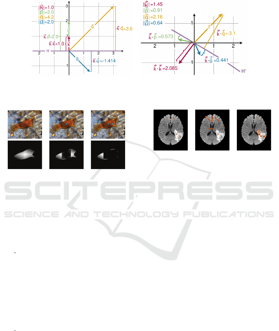
(a) (b)
Figure 3: Dot product as a similarity between vectors: (a) illustrates the hyperplane H defined by an given vector
−→
k and its
dot product to other vectors; (b) shows the same vectors after normalization.
(a) (b) (c)
Figure 4: Center-focused weight and penalization at each
iteration. Original images with estimate markers on the top,
and weight maps on the bottom. The images are cropped to
improve visualization. (a-c) Iterations 0, 1 and 2.
none of them are already part of another marker, i.e.,
∀q ∈ A
c
(p),label(q) = l,q ∈ I,q /∈ M → M
S
A
c
(p).
If the conditions are not met, the marker is not added
and another pixel must be found to be used as as
marker center. That verification function is named
valid marker() in Algorithm 1. Also, to facilitate the
extension of the markers to scribbles, a marker set
M∗ ⊂ M is created simultaneously, containing only
the center of each marker.
Extend Markers to Scribbles. Marker extension to
scribbles starts from a set of marker center M∗, an
image domain I, a ratio of increase, and an adjacency
size ρ. Then, for each marker center in the marker
set, we select a random valid direction to start the
marker growing — A direction is deemed valid if the
marker centered on the next pixel is valid according to
valid marker(). The marker grows in that direction
until it achieves half of the desired proportion, then.
The same process happens in the opposite direction in
order to respect the center of the marker (Figure 5).
In cases where the marker cannot grow until the
desired proportion, the marker selects a new direction
to keep growing. If there is no possible direction, the
bot stops without achieving the exact number. If the
(a) (b) (c)
Figure 5: Marker extension to scribbles. (a) Markers, (b-c)
scribbles for background and foreground, respectively.
early stoppage happens in the first direction, the sec-
ond one will try to compensate for the loss in size.
The algorithm goes as follows:
4.2 FLIM with Multiple Marker Sets
To learn the FLIM networks, we modify FLIM to
allow different scribble sets to learn the kernels and
the normalization parameters. As shown in Figure 6,
the training images are annotated by the marker bot,
which provides two different sets, with Scribble Set 1
being used to estimate the kernels, and Scribble Set
2 being used to learn the normalization parameters
in MBN. Multiple iterations of the Data Prep., Ker-
nel Estimation and Layer Execution are performed to
learn the FLIM encoder, which is combined with the
adaptive decoder to provide the object detection solu-
tions that are evaluated.
After the decoder, a bi-cubic interpolation scales
the output back to the original image’s domain, an
Otsu threshold binarizes the saliency, and minimum
bounding-boxes are estimated around each connected
component. In all datasets, we discard bounding
boxes with sizes smaller than 0.5% of the image’s
area to handle small noise components.
Understanding Marker-Based Normalization for FLIM Networks
617
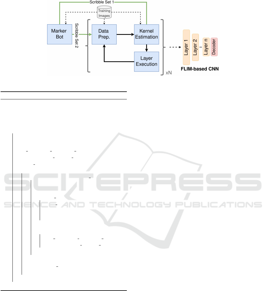
Figure 6: Pipeline for learning FLIM networks with multiple scribble sets.
Algorithm 1: Extend to scribbles.
Data: M∗,I, ratio, ρ
Result: M+
M+ ← {};
size ← len(M∗);
foreach p ∈ M do
goal ← (len(M) ∗ ratio)/2;
q ← p;
dir list = get available dir(q);
dir ← random dir(dir list);
initial dir ← dir;
for i ← 0 to 1 do
while size < goal||len(dir list) > 0 do
v ← q + dir;
m ← ad jacency(v,ρ);
if valid marker(m) then
add marker(M+,m);
q ← v;
size ← size + len(m);
end
else
dir list = get available dir();
dir ← random dir(dir list);
end
end
dir ← intial dir ∗ −1;
goal ← goal ∗ 2
end
end
4.3 Evaluation
In order to evaluate the multiple scribble sets, we pro-
pose (i) different proportions of samples in the back-
ground and foreground and (ii) analysing the impact
of the MBN along layers in the architecture of a FLIM
network. Additionally, we can analyze both (i) and
(ii) considering the decoder’s and encoder’s output
in a FLIM network. Next, we describe the proposed
evaluations when considering both outputs.
4.3.1 Decoder
Although we have an intuition of the desired fea-
ture space for convolutions, we do not know how the
normalized convolutional feature space impacts ob-
ject detection decoders. So, we propose evaluating
a FLIM CNN with adaptive decoders (as presented
in Section 6) using traditional metrics for positive
bounding box predictions. Because the decoder es-
timates the weights on the fly, it can be used in the
output of each convolutional layer, allowing an analy-
sis layer-by-layer (ii). Doing so with different sample
ratios allows us to analyze each ratio’s impact on the
decoded results (i).
4.3.2 Encoder
To evaluate the impact of (i) and (ii) in the encoder
without bias in the decoder’s quality, we propose us-
ing t-SNE (van der Maaten and Hinton, 2008) to re-
duce the many dimensions output from a convolu-
tional layer to create 2-d projections. T-SNE was se-
lected because it has shown positive results when ex-
plored to generate valuable insights about network be-
havior for human analysis(Rauber et al., 2017).
In short, consider A ∈ R
h×w×m
to be a layer’s out-
put after pooling and interpolating back to the original
image domain. T-SNE maps a sample (pixels) in the
multi-dimensional feature space to a 2-D feature vec-
tor, , for p ∈ A
′
, tSNE : p ∈ R
m
→ p
2
∈ R
2
. Then,
a color is attributed to every pixel in the new feature
space to identify whether the pixel belongs to the fore-
ground or background.
Because the projections are independent of the de-
coder’s quality, we intend to analyze them to see how
normalization impacts the resulting feature space and
if the observations correlate to the decoder results.
VISAPP 2024 - 19th International Conference on Computer Vision Theory and Applications
618

5 EXPERIMENTS
5.1 Experimental Setup
Foreground/Background Imbalancing Setups. We
ran experiments with a balanced number of samples
(1:1), a considerably imbalanced ratio (1:10, 10:1),
and a large imbalance (1:50, 50:1). For larger imbal-
ances, some images did not achieve the exact num-
ber due to lack of space inside the objects. We use
”d” to determine models that detach the normaliza-
tion marker set for each step. Therefore, if the results
state 50:1 Layer1d, we are looking at the first layer
of a model learned with different marker sets, were
for normalization, a proportion of 50:1 foreground-
to-background was used. In the detached case, the
imbalance occurred only during normalization, with
the filters being estimated with the disk markers.
Datasets. We used three dataset:
1. Schistosoma Mansoni eggs dataset (Schisto): A
proprietary microscopy dataset (Santos et al.,
2019) composed of 631 images of S. mansoni
eggs with an often cluttered background, where
the objects of interest can be partially occluded;
2. A subset of the ship detection dataset (Dadario,
2018) (Ships) composed of 463 aerial images of
ships (images out of the 621 from the original
dataset). We removed images containing ships
smaller than 1% of the image to remove the chal-
lenging drastic scale difference;
3. (Brain) A subset of a proprietary glioblastoma
dataset (Cerqueira et al., 2023) composed of 1326
slices (images out of the 44 three-dimensional im-
ages of the original dataset). The slices were ex-
tracted from the axial axis, using a stride equal to
2 and removing a percentage of removing a per-
centage of both ends (12%). The subset was com-
posed of slices of FLAIR (Fluid attenuated inver-
sion recovery) sequence of Magnetic Resonance
Imaging that shows the tumor as an active area.
Network Architecture. We fixed the same network
architecture for all datasets, and the architecture is de-
picted in Figure 7. To understand the feature spaces
created rather than finding the best model for each
dataset, we tested the decoder at the end of every layer
for every experiment. It is worth noting that all pool-
ing had a stride factor of two.
Parameters. For FLIM, the number of kernels per
marker is fixed to 5 in all layers. For the marker
bot, 5 markers were estimated for each label in each
image. The adjacency radius for marker size varied
from ρ = {4, 4,2} for the Schisto, Ships, and Brain
datasets, respectively — the variation is due to a large
size difference in the image and the objects’ areas.
Evaluation Metrics. We have two analyses of our
results: (i) The object detection results given by the
decoded features after the adaptive decoder; (2) a fea-
ture space projection analysis of the encoded features.
The former provides insight into the ratio’s impact in
networks with an adaptive decoder, and the latter eval-
uates the feature space with no decoder bias.
We propose using four distinct object detection
metrics based on positive and negative bounding
box predictions to evaluate the decoded features. A
bounding box is a positive prediction if it has an In-
tersection over Union (IoU) (Rezatofighi et al., 2019)
score greater than a threshold τ to an uncounted
ground-truth object. Based on the number of posi-
tive and negative predictions, we compute the preci-
sion and recall and derive the following metrics: the
F
2
-score, the Precision-Recall (PR) curve, the Aver-
age Precision, and the mean Average Precision. The
F
2
-score is a weighted harmonic mean of the preci-
sion and recall, favoring recall over precision. The PR
curve varies the IoU threshold to measure the achiev-
able precision for each possible recall level. The Av-
erage Precision (AP
τ
) is the Area Under the Curve of
the PR-curve up to a given threshold τ, and the Mean
Average Precision (µAP) is a good overall metric for
object detection being the mean AP over thresholds
varying from τ ∈ [0.5,0.55, ..., 0.95].
5.2 Results from Decoded Features
Considering the results for the decoded layers, Ta-
ble 1 shows the best results for each ratio setup in
each dataset. For the Schisto and Brain datasets,
foreground oversampling produced the best over-
all results; balanced sampling produced intermedi-
ate ones and background oversampling was substan-
tially worse (also seen in the PR curves in Figure
9). Oversampling creates a better representation of
individual structures within that class, and because
both datasets have considerably heterogeneous back-
grounds, the decoder highlights background objects
that activate isolated, increasing the number of false
positives (Figure 8.a-b). For the ships dataset, the best
result was achieved by oversampling the background,
although the difference was considerably less signif-
icant than it was on the other two datasets. Similar
to the previous analysis but with an opposite effect,
the oversampled class has more regions activating in-
dividually, which is detrimental for the foreground in
this dataset with higher variability of textures and col-
ors within the same object. Figure 8.c shows an ex-
ample of an event that happened with some frequency
where the object was detected but split into parts.
Regarding the impact of the markers in the nor-
Understanding Marker-Based Normalization for FLIM Networks
619
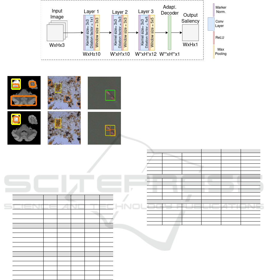
Figure 7: Architecture of trained networks.
(a) (b) (c)
Figure 8: Difference in detection predictions on different
ratios. On the top, results with a ratio of (10:1), and on the
bottom (1:10). (a-c) Brain, Schisto and Ships, respectively.
Table 1: Best results for each proportion. The two best re-
sults for each metric are in blue and green, respectively.
Schisto F
0.5
2
AP
0.5
F
0.75
2
AP
0.75
µAP
50:1 (Layer 1d) 0.744 0.663 0.530 0.280 0.364
10:1 (Layer 1d) 0.756 0.682 0.568 0.352 0.385
1:1 (Layer 1) 0.634 0.431 0.467 0.221 0.250
1:10 (Layer 2) 0.464 0.393 0.276 0.234 0.217
1:50 (Layer 2) 0.512 0.356 0.270 0.173 0.185
Ships F
0.5
2
AP
0.5
F
0.75
2
AP
0.75
µAP
50:1 (Layer 1d) 0.722 0.722 0.529 0.529 0.460
10:1 (Layer 1d) 0.740 0.743 0.517 0.518 0.464
1:1 (Layer 1) 0.764 0.770 0.564 0.568 0.503
1:10 (Layer 1d) 0.774 0.768 0.584 0.579 0.507
1:50 (Layer 1d) 0.779 0.778 0.588 0.586 0.510
Brain F
0.5
2
AP
0.5
F
0.75
2
AP
0.75
µAP
50:1 (Layer 2) 0.642 0.624 0.248 0.106 0.260
10:1 (Layer 2) 0.591 0.576 0.236 0.230 0.252
1:1 (Layer 2) 0.585 0.564 0.189 0.159 0.249
1:10 (Layer 2d) 0.094 0.059 0.017 0.002 0.019
1:50 (Layer 2) 0.398 0.355 0.105 0.058 0.135
malization alone, Table 2 shows the mean and stan-
dard deviation of all ratios for each decoded layer. A
large standard deviation means the results change sig-
nificantly depending on the ratio. That is evidence
that normalization has a meaningful impact on the
model’s performance. Also, having multiple results
from detached marker sets achieving a higher perfor-
mance than regular FLIM (Layer 1d for Schisto and
Brain and all layers from ships) indicates that using
separate marker sets might be beneficial. A combi-
nation of user-drawn scribbles for kernel learning and
their automatic extension for providing a controlled
sampling ratio could be explored for future work.
Also, note that Layer 3 had an inferior performance
in all datasets. That is primarily due to a considerable
reduction in the image size after both stridden pooling
and creating maps where the difference of mean acti-
vation was negligible, so the decoder could not per-
form correctly. A more complex decoder might be
required to exploit multiple layers better.
Table 2: Mean and standard deviation over all sampling
proportions for each layers. The two best results for each
dataset are highlighted in blue and green, respectively.
Schisto F
0.5
2
AP
0.5
F
0.75
2
AP
0.75
µAP
Layer 1 0.475±0.220 0.381±0.188 0.316±0.158 0.172±0.065 0.196±0.089
Layer 1d 0.511±0.251 0.417±0.233 0.367±0.193 0.210±0.100 0.234±0.130
Layer 2 0.548±0.069 0.419±0.064 0.319±0.039 0.183±0.028 0.214±0.024
Layer 2d 0.539±0.109 0.400±0.096 0.324±0.084 0.173±0.027 0.203±0.049
Layer 3 0.314±0.196 0.191±0.147 0.068±0.054 0.019±0.016 0.066±0.052
Layer 3d 0.304±0.162 0.181±0.129 0.062±0.051 0.024±0.020 0.064±0.050
Ships F
0.5
2
AP
0.5
F
0.75
2
AP
0.75
µAP
Layer 1 0.745±0.015 0.702±0.086 0.506±0.060 0.404±0.176 0.403±0.096
Layer 1d 0.756±0.022 0.756±0.021 0.556±0.029 0.556±0.027 0.489±0.022
Layer 2 0.553±0.114 0.501±0.140 0.282±0.144 0.201±0.194 0.231±0.123
Layer 2d 0.575±0.094 0.504±0.148 0.321±0.115 0.244±0.172 0.251±0.128
Layer 3 0.282±0.145 0.229±0.172 0.071±0.047 0.013±0.010 0.071±0.058
Layer 3d 0.328±0.145 0.242±0.200 0.094±0.049 0.021±0.012 0.079±0.069
Brain F
0.5
2
AP
0.5
F
0.75
2
AP
0.75
µAP
Layer 1 0.178±0.129 0.147±0.132 0.055±0.041 0.033±0.029 0.063±0.054
Layer 1d 0.269±0.146 0.211±0.130 0.099±0.072 0.038±0.032 0.085±0.053
Layer 2 0.459±0.207 0.428±0.223 0.159±0.087 0.111±0.079 0.181±0.098
Layer 2d 0.345±0.163 0.315±0.167 0.115±0.061 0.090±0.061 0.132±0.077
Layer 3 0.030±0.031 0.011±0.014 0.003±0.004 0.000±0.000 0.002±0.003
Layer 3d 0.034±0.032 0.011±0.014 0.003±0.004 0.000±0.000 0.002±0.003
As presented in Table 3, the variance among
different layers considering the same foreground-to-
background proportion is not very high for the ra-
tios that provided an adequate result (blue and green),
apart from the F
0.5
and AP
0.5
in the brain dataset.
That is likely because this dataset is more challeng-
ing, and appropriate solutions are achieved only at the
second layer, resulting in a significant difference in
results. In most images of that dataset, layer one can
detect only a partial part of the tumor, while Layer 2
has a much more homogeneous activation.
The ships dataset had the most negligible impact
among different setups (also in Table 3) where over-
sampling the background was better than doing it for
the foreground. That is likely due to the homogeneity
of the background within most images in the dataset,
making it easier to isolate non-background regions by
better characterizing the background instead of isolat-
ing regions with high similarity to the foreground.
VISAPP 2024 - 19th International Conference on Computer Vision Theory and Applications
620
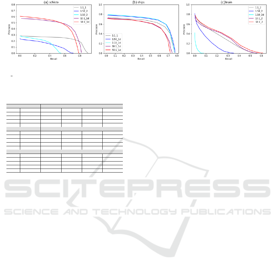
Figure 9: Precision-Recall curves for each dataset considering the best performing layer for each sampling ratio. In the caption
1:10 1d means the results come from 1:10 proportion, layer 1 and detached marker sets. (a) Schisto; (b) Ships; (c) Brain.
Table 3: Mean and standard deviation of Layers 1, 1d, 2, 2d
for each sampling proportion. The two best results for each
metric in each dataset are in blue and green, respectively.
Schisto F
0.5
2
AP
0.5
F
0.75
2
AP
0.75
µAP
50:1 0.681±0.036 0.575±0.052 0.427±0.063 0.216±0.046 0.290±0.043
10:1 0.667±0.058 0.545±0.095 0.449±0.076 0.234±0.071 0.280±0.064
1:1 0.574±0.060 0.401±0.030 0.398±0.069 0.200±0.021 0.222±0.028
1:10 0.289±0.133 0.225±0.119 0.172±0.072 0.129±0.066 0.120±0.064
1:50 0.381±0.120 0.275±0.069 0.210±0.056 0.144±0.023 0.146±0.032
Ships F
0.5
2
AP
0.5
F
0.75
2
AP
0.75
µAP
50:1 0.583±0.142 0.570±0.153 0.335±0.176 0.226±0.191 0.273±0.137
10:1 0.607±0.136 0.517±0.145 0.320±0.151 0.201±0.188 0.243±0.136
1:1 0.649±0.114 0.560±0.210 0.412±0.152 0.327±0.241 0.323±0.181
1:10 0.724±0.042 0.716±0.046 0.520±0.058 0.513±0.061 0.450±0.047
1:50 0.723±0.039 0.716±0.042 0.495±0.058 0.490±0.061 0.429±0.054
Brain F
0.5
2
AP
0.5
F
0.75
2
AP
0.75
µAP
50:1 0.394±0.182 0.350±0.188 0.163±0.064 0.091±0.045 0.148±0.077
10:1 0.333±0.213 0.296±0.206 0.128±0.088 0.096±0.084 0.124±0.090
1:1 0.458±0.127 0.438±0.126 0.152±0.036 0.116±0.043 0.191±0.058
1:10 0.078±0.014 0.025±0.021 0.014±0.004 0.001±0.001 0.008±0.007
1:50 0.302±0.095 0.267±0.087 0.077±0.035 0.036±0.022 0.105±0.032
5.3 Feature Projection Analysis
Analyzing all possible combinations of feature spaces
from the proposed experiments of Sec. 5.2 would be
unfeasible. For each dataset, we proposed to evalu-
ate five foreground and background proportions (50:1,
10:1, 1:1, 1:10, and 1:50) and feature spaces of the
output of three distinct layers. Additionally, each
dataset contains hundreds of samples, and each im-
age contains thousands of pixels. Projecting pixels
of all images in a dataset would result in a projection
with millions of points. Due to that, we select one
image from the experiment with a large variation in
F
0.5
2
among layers and sample ratio. We then project
the encoder’s output related to this image in the 2D
space. Results for both comparisons are given below.
5.3.1 Different Foreground-to-Background
Ratio
Image-space projections of one image per dataset are
shown in Figure 10. Blue points are foreground pix-
els, and red points are background. For each dataset
(rows), different proportions for background and fore-
ground markers are presented (columns).
For Schisto, one can notice a big and dense cloud
of background points with some foreground ones
mixed into the cloud (in the middle right of the large
cloud). For 50:1, 10:1, and 1:1, a small group of
red points is separated from the blue cloud while an-
other is attached. For 1:10 and 1:50, there is no clear
separation between the blue cloud of points and any
group of red points. This visual hint is confirmed by
the quantitative results obtained by the decoder in Ta-
ble 3, which shows better results for proportions of
50:1 and 10:1.
For Schips, a big and dense cloud of blue points
(background) is entirely separated from a small group
of red points (foreground). There is no mixture be-
tween red and blue points in the projections. Again,
this visual hint agrees with the quantitative results
obtained by the decoder in Table 3, but the non-
substantial increase in background oversampling is
most likely due to decoder limitations rather than a
less suitable feature space.
For Brain, a semi-circle of blue points and some
groups of blue points are observed in all projections
of distinct proportions. Also, there is a group of red
points in the tail of the semi-circle of the blue points.
For 50:1 and 10:1, the group of red points is more
compact. Particularly, for 1:10, the spread of red
points over the semi-circle of blue points is larger.
That also agrees with the results in Table 3.
Additionally, analysing distinct datasets, the pro-
jections with a clear separation between classes are
the ones that provided better results for the object de-
tection metric, where Ships had the highest results,
followed by Schisto and lastly Brain.
5.3.2 Along Layers
Figure 11 shows image space projections of one im-
age per dataset. For distinct datasets (rows), the out-
put of distinct layers is presented (columns).
For Schisto and Ships, a dense cloud of blue points
is separated from a small group of red points in layer
1, although there is more mixture of red points in the
bottom right of the blue cloud for the Schisto dataset.
On layer 2, Schisto still presents a similar separation
to the first layer, but there is more mixture for Ships.
These observations align with the average behavior
described in Table 2, where the results from the first
Understanding Marker-Based Normalization for FLIM Networks
621
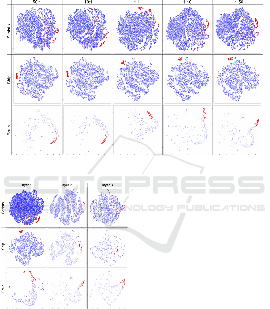
Figure 10: 2D projected image spaces for a single image in each dataset. Each point in the projection refers to a pixel whose
color indicates whether it is from the background (blue) or foreground (red). Opacity of blue samples is set to show the
number of samples overlapping.
Figure 11: 2D projected image spaces for a single image in
each dataset and for different layers. Each point refers to
a pixel whose color indicates whether it is from the back-
ground (blue) or foreground (red). Opacity of blue samples
is set to show the number of samples overlapping.
two layers are similar for the Schisto dataset but a
larger degradation for the second layer on Ships. In
layer 3, the separation is no longer seen in either case.
For Brain, in layer 1, most blue points are grouped
in a semi-circle with a tail of red points with no clear
separation between them, and small groups of isolated
red and blue points are seen. In layer 2, red points
are in a single and more clustered group, with less
mixture among red and blue points compared to the
other layers, which was the layer with better results
in Table 2. No semi-circle structure of blue points is
present in layer 3, as seen in the other layers. Red
points are also more spread out and not in a dense and
small group.
Also, when comparing projections for distinct
datasets, one can notice that the best projection for
any layer – in which red groups (foreground) are more
separated from blue points (background) – is given
by Ship, layer 1, Schisto, layer 2, and Brain, layer
2 in this order, which is in line with the best quan-
titative results for the decoder evaluation in Table 1.
The visual separation between foreground and back-
ground points in the 2D projection also follows the
same trend as the adaptative decoder. As a result, this
experiment shows a positive correlation between the
separation of points of foreground and background of
distinct layers in a 2D projection and qualitative re-
sults of an adaptative decoder.
VISAPP 2024 - 19th International Conference on Computer Vision Theory and Applications
622

6 CONCLUSION
We evaluated the impact of different marker sets when
learning the normalization parameters of FLIM net-
works for object detection. For this analysis, we mod-
ified the FLIM methodology to allow one marker set
to be used when estimating the kernels and another
when computing the normalization parameters. We
also introduced a marker bot to create FLIM CNNs
automatically from ground truth with a desired pro-
portion of foreground-to-background ratio.
Our analysis showed a positive correlation be-
tween 2D projections and our adaptive decoder, open-
ing ways to build encoders more suitable for FLIM
networks without needing a decoder for layer evalua-
tion. The results showed that different normalization
parameters have significant impact and oversampled
classes provide a better representation of their object
parts, allowing the design of a more accurate, high-
quality, and interpretable FLIM network.
For future work, user-drawn markers could be
used to create better-positioned markers for learning
the kernels, and then they could be extended automat-
ically to learn the normalization parameters in the de-
sirable unbalanced setup to provide better solutions.
Also, a similar study could be developed with the de-
tached marker sets to understand better the impact of
different markers for kernel estimation, having a fixed
set for normalization.
ACKNOWLEDGEMENTS
The authors thank the financial support from
Coordenac¸
˜
ao de Aperfeic¸oamento de Pessoal de
N
´
ıvel Superior – Brasil (CAPES) with Finance
Code 001, CAPES COFECUB (88887.800167/2022-
00), CNPq (303808/2018-7), FAEPEX, and Labex
B
´
ezout/ANR.
REFERENCES
Cerqueira, M. A., Sprenger, F., Teixeira, B. C., and Falc
˜
ao,
A. X. (2023). Building brain tumor segmentation net-
works with user-assisted filter estimation and selec-
tion. In 18th International Symposium on Medical
Information Processing and Analysis, volume 12567,
pages 202–211. SPIE.
Dadario, A. M. V. (2018). Ship detection from aerial im-
ages. https://www.kaggle.com/datasets/andrewmvd/
ship-detection.
De Souza, I. E. and Falc
˜
ao, A. X. (2020). Learning cnn fil-
ters from user-drawn image markers for coconut-tree
image classification. IEEE Geoscience and Remote
Sensing Letters.
Jain, A., Nandakumar, K., and Ross, A. (2005). Score nor-
malization in multimodal biometric systems. Pattern
recognition, 38(12):2270–2285.
Joao, L. d. M., Santos, B. M. d., Guimaraes, S. J. F.,
Gomes, J. F., Kijak, E., Falcao, A. X., et al.
(2023). A flyweight cnn with adaptive decoder for
schistosoma mansoni egg detection. arXiv preprint
arXiv:2306.14840.
Kaur, J. and Singh, W. (2022). Tools, techniques, datasets
and application areas for object detection in an im-
age: a review. Multimedia Tools and Applications,
81(27):38297–38351.
MacQueen, J. et al. (1967). Some methods for classification
and analysis of multivariate observations. In Proceed-
ings of the fifth Berkeley symposium on mathematical
statistics and probability, volume 1, pages 281–297.
Oakland, CA, USA.
Nair, V. and Hinton, G. E. (2010). Rectified linear units
improve restricted boltzmann machines. In Proceed-
ings of the 27th international conference on machine
learning (ICML-10), pages 807–814.
Omar, N., Supriyanto, E., Wahab, A. A., Al-Ashwal, R.
H. A., and Nazirun, N. N. N. (2022). Application of k-
means algorithm on normalized and standardized data
for type 2 diabetes subclusters. In 2022 International
Conference on Healthcare Engineering (ICHE), pages
1–6. IEEE.
Rauber, P. E., Fadel, S. G., Falc
˜
ao, A. X., and Telea, A.
(2017). Visualizing the hidden activity of artificial
neural networks. IEEE TVCG, 23(1).
Rezatofighi, H., Tsoi, N., Gwak, J., Sadeghian, A., Reid, I.,
and Savarese, S. (2019). Generalized intersection over
union: A metric and a loss for bounding box regres-
sion. In Proceedings of the IEEE/CVF conference on
computer vision and pattern recognition, pages 658–
666.
Santos, B. M., Soares, F. A., Rosa, S. L., Gomes, D. d. C. F.,
Oliveira, B. C. M., Peixinho, A. Z., Suzuki, C. T. N.,
Bresciani, K. D. S., Falcao, A. X., and Gomes, J. F.
(2019). Tf-test quantified: a new technique for diag-
nosis of schistosoma mansoni eggs. Tropical Medicine
& International Health.
Sousa, A. M., Reis, F., Zerbini, R., Comba, J. L., and
Falc
˜
ao, A. X. (2021). Cnn filter learning from drawn
markers for the detection of suggestive signs of covid-
19 in ct images. In 2021 43rd Annual International
Conference of the IEEE Engineering in Medicine &
Biology Society (EMBC).
van der Maaten, L. and Hinton, G. (2008). Visualizing data
using t-SNE. JMLR, 9:2579–2605.
Zaidi, S. S. A., Ansari, M. S., Aslam, A., Kanwal, N., As-
ghar, M., and Lee, B. (2022). A survey of modern
deep learning based object detection models. Digital
Signal Processing, page 103514.
Zeiler, M. D., Fergus, R., Fleet, D., Pajdla, T., Schiele,
B., and Tuytelaars, T. (2014). Visualizing and Un-
derstanding Convolutional Networks, pages 818–833.
Springer International Publishing, Cham.
Understanding Marker-Based Normalization for FLIM Networks
623
