Between Gaming and Microclimate Simulations: Temperature

Estimation of an Urban Area

Eva Strauss and Dimitri Bulatov

Fraunhofer Institute for Optronics, System Technologies and Image Exploitation (IOSB),

Gutleuthausstrasse 1, 76275 Ettlingen, Germany

Keywords:

Urban Heat Island, Thermal Simulation, Digital Twin, 3D City Model, Thermal Remote Sensing.

Abstract:

With the rising awareness and interest from researchers, local authorities, and industry in the urban heat island

effect, thermal remote sensing data is needed as it allows for identiﬁcation, tracking, or analysis of land sur-

face temperatures. Yet, the accessibility of appropriate thermal data in both the spatial and temporal domain

states an inhibiting factor. Whilst thermal satellite data suffers from both low spatial and temporal resolution,

airborne imagery might enable adequate resolutions, however, is not acquired without time and cost consump-

tion. One way to overcome this drawback is the generation of synthetic data, which comprises the simulation

of surface temperatures. These rather simpliﬁed simulations are either quite fast, as desired in gaming applica-

tions, however, highly inaccurate, or rather complex, holistic, time-consuming and computationally intensive,

like applied in urban microclimate considerations. In this paper, we present an in-between approach towards

the estimation of urban surface temperatures that aims to ﬁll this gap between holistic microclimate simula-

tions and climate maps.

1 INTRODUCTION

1.1 Motiviation

In the last century, the world-wide urbanization de-

gree increased tremendously, and by 2050, the por-

tion of people living in cities or urbanized areas is

expected to be almost 70%. With the concurrent in-

crease of summer heat periods, researcher, local au-

thorities and industry became aware of the need to

maintain the city as a livable area by taking coun-

termeasures against the so-called urban heat island

(UHI) effect. This effect describes the overall higher

temperatures of urban areas compared to their rural

surroundings. Its cause is found in cityscapes, con-

struction materials and type, latent factors like popu-

lation density or trafﬁc, and others. Therefore, many

countermeasures currently applied or under research

evolve around these causes, and interest in computer-

aided tools to quantify the actual effect of counter-

measures is growing. One such computer-aided tool

is given by urban climate simulation software. There,

heat transport and ﬂow dynamics are usually consid-

ered, which makes the overall simulation a complex,

https://orcid.org/0000-0002-0560-2591

time-consuming task requiring interdisciplinary ex-

pert knowledge. Thus, it is not feasible for, e.g., archi-

tects or urban planners who seek rather fast and easy

to generate as well easy to interpret results. Looking

for a faster way to simulate the temperature distribu-

tion of an urban area, one might look into the area of

gaming and physics-based sensor simulations. Here,

simulation runtimes are drastically reduced up to re-

altime, however, stream dynamics are not taken into

account. In other words, the ﬂow and temperature of

air through a city, its convective cooling and its ef-

fect on human comfort, which is generally of essence,

are not considered. Last but not least, climate maps

state another very fast option to estimate local ur-

ban climate. No differential equations need to be nu-

merically solved, instead, urban areas are segmented

by their local climate solely depending on land-use,

vertical roughness, topography, portion of water bod-

ies, and similar features. In summary, a large gap in

accuracy between near real-time climate estimations

and holistic micro-climate simulations can be iden-

tiﬁed by the urban planners. To bridge the gap, a

tool for a quick, superﬁcial screening of a large ur-

ban scene is required allowing to detect potential ar-

eas of urban heat accumulation. For a few candidates

of (smaller) areas particularly vulnerable to UHIs, a

Strauss, E. and Bulatov, D.

Between Gaming and Microclimate Simulations: Temperature Estimation of an Urban Area.

DOI: 10.5220/0012385800003660

Paper published under CC license (CC BY-NC-ND 4.0)

In Proceedings of the 19th International Joint Conference on Computer Vision, Imaging and Computer Graphics Theory and Applications (VISIGRAPP 2024) - Volume 1: GRAPP, HUCAPP

and IVAPP, pages 70-80

ISBN: 978-989-758-679-8; ISSN: 2184-4321

comprehensive micro-climate simulation can be then

launched, thus allowing to save time and computa-

tional resources. In this paper, we present an in-

between approach towards surface temperature sim-

ulation serving as previously mentioned tool. We par-

ticularly address the physical modeling of the heat

transfer. Thus in this context, the proposed methods

are more sophisticated than gaming approaches, yet

signiﬁcantly simpliﬁed in direct comparison to micro-

climate simulations.

The rest of the paper is organized as follows: To

systematize the state of the art on available tools on

thermal simulation, we provide a concise overview of

current simulation methods and software in Section

1.2 and an introduction to the base simulation frame-

work we built up on in Section 2.1. Afterwards, we

present our methods of choice in Section 2, which

is followed by the evaluation of our methods in Sec-

tion 3. Finally, we summarize our ﬁndings and future

work in Section 4.

1.2 Related Work

While the UHI describes temperature increase of

cities in comparison to their rural surrounding, the

microclimate generally refers to the ground-level cli-

mate inﬂuenced by the physical characteristics of the

present surfaces. An alternative to laborious and

costly inner-city measurements is provided by micro-

climate simulations. They make it possible to cover

large areas, analyze the impact of city design on UHI

formation and even thermal comfort. One quite well-

known commercial software for microclimate simula-

tions is ENVI-met (Liu et al., 2021). This tool allows

for simulation of single building (yet no interior),

city quarters or whole smaller cities. Designed as a

holistic approach, each physical phenomenon inﬂu-

encing the microclimate is modeled, including radia-

tive heat exchange, photosynthesis, and evapotranspi-

ration. Another simulation tool under ongoing devel-

opment is PALM-4U. As research project under na-

tional funding by the German Federal Ministry of Ed-

ucation and Research (BMBF), the open-source soft-

ware is designed to help in municipal adaption strate-

gies concerning the UHI and other climate-related

changes in urban areas. It offers a higher resolution in

turbulences and is highly parallelized. With PALM-

4U, it is aimed for usability in civil service and public

authority. Envi-met and PALM-4U, as usual microcli-

mate simulation tools, are based on continuous ﬂuid

dynamics (CFD) to numerically solve for the temper-

ature and wind ﬁelds. They provide great accuracy,

yet by their CFD nature, they are time-consuming and

demanding, require expertise in the ﬁeld of numerical

simulation and thus speciﬁc training.

Other simulations frameworks focus on speciﬁc

tasks or reduced scale, such as building energy tools

for single building simulation. They provide great de-

tail on an appropriate scale, yet cannot be extended to

the urban city scale without huge drawbacks in com-

putation time and cost. Thus, to overcome the gap

between precise building energy simulation (BES)

and CFD on urban areas, BES-CFD coupling tech-

niques have been researched (Rodr

ıguez-V

azquez,

Martin and Hern

andez-P

erez, Iv

an and Xam

an, Je-

sus and Ch

avez, Yvonne and Gij

on-Rivera, Miguel

and Belman-Flores, Juan M., 2020; Ruijun Zhang,

2021). Bringing together the respective advantages,

high computation time and cost still remains.

Shifting the point of view from microclimate sim-

ulation tools towards scene generation and more game

oriented tools, such as the software components by

Presagis (Presagis, 2023) or Oktal-SE (Oktal-SE,

2023), a paradigm change can be observed. Instead

of expensive CFD simulation, these tools mostly rely

on highly simpliﬁed surface temperature simulation

and rather focus sophisticated camera models. Thus,

they clearly outperform microclimate simulations in

terms of runtime and computational cost, yet to the

extent of accuracy.

Motivated and inspired from the above method-

ologies to urban temperatures, our approach aims at

converging these by picking and combining respec-

tive models and thus yielding reliable results with ap-

propriate computation time, cost, and accuracy.

2 METHODOLOGY

2.1 Preliminaries

The heat distribution of an urban area depends on

many factors, which makes its computation a chal-

lenging task. These factors include, but are not lim-

ited to: construction materials and geometries, cli-

mate conditions (both macro- and micro-climate), lo-

cal weather conditions and weather history over a

larger time span, as well as factors depending on the

residents, like population or trafﬁc. Each of these

contributes to the generation or transfer of heat and

raises the need for a huge amount of information

given prior to climate simulations. A so-called dig-

ital twin, which combines 3D geometry with addi-

tional information, states a great starting point for ur-

ban temperature estimation. In this paper, we focus

on the cityscape and construction materials, and refer

to the digital twin as the 3D reconstruction of an ur-

ban area, in form of a triangle mesh, with semantic

Between Gaming and Microclimate Simulations: Temperature Estimation of an Urban Area

and material information. Since the aerial data pro-

vide the most cost-efﬁcient method to derive the most

essential information from large scene, we followed

the procedure of (Bulatov et al., 2020) to generate the

digital twin from a high-resolution orthophoto, a nor-

malized digital surface model (ndsm), multi-spectral

imagery, and OSM data. In a nutshell, an index is

assigned by semantic segmentation and material clas-

siﬁcation to each triangle representing its semantic

type (ground, building part or vegetation), its mate-

rial type (i.e. street, grass, soil, or water for ground

triangles, roof or wall for buildings, and forest, decid-

uous tree, shrub or palm tree for vegetation), as well

as color (image-derived for visible and geo-typical for

non-visible, such as building walls, objects). These

indices are linked to a material database where physi-

cal parameters like density, heat conductivity, or spe-

ciﬁc heat capacity, needed for temperature calcula-

tion, are stored. Currently considered material classes

are street, grass, soil, water, building roof, building

wall, vegetation.

2.2 Overview of Thermal Simulation

The starting point of our proposed thermal simulation

framework is given by the 3D semantic city model,

i.e. the three-dimensional triangular mesh with dis-

tinct numeric class labels per triangle, as described

in Sec. 2.1. Environmental data needed for the sim-

ulation, including wind speed, air temperature, or

relative humidity, is considered to be available via

weather stations nearby the city to be simulated. Due

to thermal inertia, a minimum time-span of 48h has

to be simulated, such that corresponding weather data

has to be gathered. Generally, we calculate the surface

temperatures based on the well-known heat equation

applied to the full scene. To do so, a ﬁnite volume

method (FVM) is deployed by expanding each sur-

face triangle of the 3D mesh into a prism of material-

dependent depth which is sliced into several layers

following (Kottler et al., 2019). Here and in the fol-

lowing, we will refer to this as the surface volume.

For each layer, average temperatures are estimated

by modeling the net heat ﬂux. Thus, the surface layer

is affected by convective, radiative and conductive

heat, while the inner layers only experience heat con-

duction. Due to its high complexity, latent heat is not

yet regarded in the presented work. Following (Kot-

tler et al., 2019; Bartos and Stein, 2015), the temporal

temperature evolution for each surface layer is given

v,s

∂T

∂t

= q

conv

+ q

s,cond

+ γ

sky

rad

+ γ

sun

sol

(1)

with the temperature of the surface T

, the solar short-

wave heat ﬂux q

sol

, the radiative long-wave heat ﬂux

rad

, the factors γ

sun

∈ [0; 1] yielding weather the sur-

face layer is exposed to sunlight and γ

sky

∈ [0; 1] yield-

ing the relative exposure to the sky in orthogonal di-

rection, the conductive heat ﬂux q

cond

, the convective

heat ﬂux q

conv

, the material-dependent speciﬁc heat

capacity c

v,s

and material density ρ

of the surface

layer, and ﬁnally its depth d. The inner layers, i.e.

below the surface, only experience conductive heat

transfer, yielding

v,i

∂T

∂t

= q

i,cond

(2)

where i indicates the i-th layer with corresponding

heat ﬂux q

i,cond

and temperature T

, and it is i =

1...(n − 1) with n being the number of layers. The

layer depths are assumed to be equal. Depending on

the present semantic class and material of the surface

element, we set the temperature of the last layer to a

constant, or assume the heat ﬂux to be zero, i.e. some

kind of insulation being apparent in the semantic ob-

ject. In the following, details on the heat ﬂux terms

will be outlined.

2.3 Conductive Heat

The individual layers of a given surface volume are

assumed to exchange heat by conduction following

Fourier’s law. Furthermore, we assume a lateral heat

exchange between surface volumes, in particular be-

tween neighboring layers, see Figure 1.

Thus the conductive ﬂuxes in Eq. (1) and ((2)) are

s,cond

− T

)

∑

j∈N

s j

(∇T )

s j

⃗n

s j

(3)

i,cond

−

i−1

− T

)

i+1

− T

)

∑

j∈N

i j

(∇T )

i j

⃗n

s j

(4)

with the area A of the surface triangle, its set of neigh-

boring triangles N

, and the length L

s j

and normal⃗n

s j

of the corresponding edge between the surface and the

neighboring triangle indexed vy j. It is ⃗n

i j

=⃗n

s j

and

i j

= L

s j

for all sub-surface layers i. Hence, (∇T )

i j

denotes the derivative in direction of⃗n

s j

. The conduc-

tivity at layer interfaces, denoted by k

and k

i j

, are

determined as min(k

i±1

) and min(k

), respec-

tively. As previously stated, we set the boundary con-

ditions on the last layer denoted by n depending on

the surface triangles’ semantic class, i.e.

GRAPP 2024 - 19th International Conference on Computer Graphics Theory and Applications



(∇T )

= 0 if building roof or wall

= const. otherwise

(5)

where (∇T )

denotes the derivative of T along the

surface normal.

Figure 1: 3D surface volumes. Colors indicate the material

classes street (gray), gras (green), soil (brown), and user-

deﬁned (magenta). Blue arrays indicate direction of con-

ductive heat transfer.

Ground

Roof

Wall

Gras Layer

Water Layer

Street Layer

Soil Layer

Insulation Layer: No Heat Transfer

Core Layer: Constant Temperature

Figure 2: Schematic representation of the material compo-

sition per surface class.

Given the numeric semantic class label of the

surface triangles, material properties being needed

in above equations are deduced. Namely, these are

density, speciﬁc heat capacity, and heat conductiv-

ity. The class label serves as unique identiﬁer refer-

encing to the material library holding these parame-

ters. However, since only the surface class is known,

sub-surface materials have to be approximated. The

authors of (Kottler et al., 2019) applied the proper-

ties of the surface triangle also on sub-surface lay-

ers, while commercial software tools such as Envi-

met (Liu et al., 2021) provide more sophisticated de-

fault compositions of material layers. Yet, case stud-

ies using microclimate simulation software often re-

veal the need for manual adaption of materials to

make them a better ﬁt to reality. In our model, we

thus provide default as well as adaptable 1D surface

volumes. These are deﬁned as an array of materials

each with corresponding depth boundaries. The ma-

terials are uniquely identiﬁed by a numerical value,

referencing again the given material library. By de-

fault, given the unique surface materials of a semantic

3D city model, the 1D surface volumes are automat-

ically generated and, according to the ﬁrst material

in the array, i.e. the surface material, assigned to the

corresponding triangle of the 3D city model. Alter-

natively, a semi-automatic process can be employed,

where 1D surface volumes are manually deﬁned and

automatically assigned to the 3D city model. Figure

1 illustrates the 3D surface volume with directions of

heat conduction, and Figure 2 displays the boundary

conditions and materials assigned by default to the 1D

surface volume.

2.4 Convective Heat

Convection describes the transfer of heat by a moving

ﬂuid, such as air or water, and distinction is made be-

tween natural convection, where a ﬂuid starts moving

due to a change in temperature, and forced convec-

tion, where a temperature change occurs due to forced

ﬂuid motion by an external source, e.g. wind or ven-

tilators. In an outdoor scene, an example for natural

convection is the visible rising air directly above hot

streets during summer heat periods. Yet, natural con-

vection often is exceeded by forced convection due

to wind movement. Generally, the convective heat

ﬂux is proportional to the temperature difference of

a given surface and the moving ﬂuid. Introducing the

convective heat transfer coefﬁcient (CHTC), the con-

vective heat ﬂux in Eq. (1) is given by

s,conv

= h(T

air

− T

) (6)

with the CHTC h. Generally, the estimation of h is

a tremendously challenging task. Particularly within

a city, dependencies on cityscape, material properties

such as roughness or coating, wind speed and many

others occur. Corresponding research usually focuses

on very speciﬁc situations under well-deﬁned condi-

tions. For this reason, we chose a CHTC model that

takes into account the 3D geometry of the city model

and is based on CFD simulations following (Awol

et al., 2020). Therein, the authors propose three new

correlations which set into relation the wind speed at

10m height above ground, the building packing den-

sity, and the ﬂow regime. The authors differentiate be-

tween the isolated (large distance between buildings

compared to their height) and interference/skimming

(medium to low distance between buildings compared

to their height) regimes. They further assume ideal

cubic buildings uniformly spread on an orthogonal

grid. The proposed correlations from (Awol et al.,

2020) are given in the form of

h = c

· v

· (c

· λ

− c

· λ + 1) (7)

in the isolated ﬂow regime and

h = c

· v

· (c

− c

· λ) (8)

in the interference/skimming ﬂow regime, with the

wind speed at 10m height above ground v

and the

packing density λ of the buildings. The parameters c

Between Gaming and Microclimate Simulations: Temperature Estimation of an Urban Area

, c

, and c

depend on the relative surface ori-

entations clustered in the four categories windward,

top, lateral and leeward. To apply the proposed cor-

relation to our case, a triangle-wise estimation of the

building packing density, the ﬂow regime, and the rel-

ative surface orientation category has to be carried

out. We hold on to the assumption of cubic buildings

and thus estimate the building packing density as

λ =

(9)

with A

the summarized planar area of all buildings

in the scene and A

the not built-up area, yet involv-

ing all ground surfaces, including streets or pavement.

The planar areas A

and A

are yielded by the orthog-

onal projection of the 3D city model with its semantic

class labels. We further estimate the ﬂow regime by

the percentage of the built-up area with respect to the

full scene and neglect differences in building heights.

Given the LOD1 buildings, each roof triangle is as-

signed the category top of the relative surface orien-

tation. By taking the dot product of surface normals

and wind direction, which is assumed to be constant

in space and time, wall triangles are assigned the cor-

responding categories windward, lateral, or leeward.

Since the correlations given by Eq. (7) and (8) are

only valid for buildings, another CHTC model has to

be used for ground and vegetation. At ground, par-

allel laminar ﬂow is assumed, and from (Energie und

Umwelttechnik, 2009), we formally set the CHTC to

h =

(

7.3v

0.73

, if v

> 5 m/s

1.8 + 4.1v

, otherwise

(10)

depending on the wind speed, i.e. whether forced con-

vection outperforms natural convection or not.

The CHTC model above is valid for building tri-

angles, yet ground and vegetation triangles have to be

considered separately. Vegetation further raises the

challenge in thermal modeling due to their active na-

ture, as it actively regulates its temperature via evapo-

transpiration to a certain degree (Kibler et al., 2023).

In our approach, we assume the temperature of vege-

tation to be equal to air temperature. Thus, latent heat

accounting for the effect of transpiration and evapo-

ration from vegetation as well as moist ground is not

included in our model for the sake of simplicity.

2.5 Radiative Heat

Radiative heat exchange in an urban area can be sepa-

rated in heating due to solar exposure, heat exchange

between objects, and exchange between surfaces and

the surrounding atmosphere. While the ﬁrst partic-

ularly occurs due to the short-wave infrared radia-

tion within the solar spectrum, the latter two occur

in the long-wave infrared spectrum, which is also

known as thermal radiation and strongly depends on

the scenery, namely the surface materials, surface ar-

eas and their mutual exposure.

We formally follow (Kottler et al., 2019; Bulatov

et al., 2020) to model both radiative heat ﬂuxes. Thus,

the solar heat ﬂux q

sol

on an exposed surface oriented

by the angle φ in direction of the incoming sunlight is

given by

sol

= (1 − a)E

cos(φ) (11)

with the color-dependent solar albedo a, i.e. the so-

lar reﬂectance of the surface, and the solar irradia-

tion E

at the surface, i.e. damped by the atmosphere.

The sky is mathematically assumed as inﬁnite surface

with a corresponding sky temperature T

sky

yielding

the long-wave radiative heat ﬂux

rad

= σε(T

sky

− T

) (12)

with the emissivity ε of the surface material and the

Stefan-Boltzmann constant σ.

2.6 Initial Condition

The numerical estimation of temperatures in transient

heat transfer states an initial value problem and due

to thermal inertia, the initial temperature distribution

is crucial and affects the temporal temperature evolu-

tion. This is why the simulation of temperatures of

a 3D city model at a given point in time should al-

ways include the simulation of temperatures for a pre-

ceding time span, from a few hours up to a few days

depending on the chosen initial temperatures. When

measured temperature distributions are given, the pre-

ceding simulation time can be minimized. Our over-

all simulation framework was thus designed to allow

for aerial thermal imagery to be used as initial data,

whereas unseen structures are interpolated. For ex-

ample, these might be walls, windows, or tree trunks.

If no measured data is available, a 1D precalculation,

i.e. no lateral heat conduction, of material-wise tem-

peratures is performed. In other words, the 1D tem-

perature distribution of each unique surface volume is

independently simulated. Each surface volume is as-

sumed to represent a ﬂat triangle with no elevation nor

shadowing, the environmental conditions are given by

the ﬁrst 24 hours of the overall timespan to be simu-

lated, and the ﬁrst air temperature entry serves as ini-

tial temperature.

2.7 Thermal Radiance for

Image-to-Image Comparison

Generally, when an aerial thermal image is provided,

measured surface temperatures need to be deduced.

GRAPP 2024 - 19th International Conference on Computer Graphics Theory and Applications

Since any thermal camera generally measures heat

radiance instead of actual temperatures, the cameras

sensor output is translated into temperature values by

some approximations either within the camera or by

camera-speciﬁc tools. Yet, the underlying correla-

tions, applied approximations and speciﬁcations are

usually company property, thus not publicly available

and often not provided. To compare the simulated sur-

face temperatures against thermal imagery, we thus

consider not only the simulated surface temperatures

themselves but also the simulated heat radiance for

better image-to-image comparability. Given the simu-

lated surface temperatures T

, this radiance is approx-

imated by

L = ε

(λ,T

)dλ whereby

(λ,T ) =



exp



λ · T



− 1



−1

(13)

with the material-wise thermal emissivity ε, integra-

tion over the long-wave infrared spectrum with λ

8µm and λ

= 14µm, and the spectral radiance fol-

lowing Planck’s law with constants c

and c

. The in-

tegral can be solved numerically by transforming into

a fast converging series, yielding (Wallrabe, 2001)

L = ε

[S(x

) − S(x

)] whereby

S(x

) =

∞

∑

i=1

(ix

)

+ 3(ix

)

+ 6ix

+ 6

exp(ix

)

with x

for n = 1, 2.

(14)

To keep the radiance model as simple as possible,

atmospheric or sensor-speciﬁc effects are not mod-

eled. With simulated temperature and radiance values

per triangle, a simple OpenGL rendering is performed

in order to generate simulated images of the area in

correspondence to the measured thermal image.

3 RESULTS

The simulation approach has been carried out for an

urban area in the City of Melville, Western Australia.

The reconstructed area of size 2 km × 1 km is shown

in Figure 3. The reconstruction as discussed in Sec.

2.1 is a triangle mesh with semantics and materi-

als assigned. This mesh consists of 1648685 trian-

gles. Hereby, buildings are given with level-of-detail

(LOD) 1 while the vegetation is represented either

as a standard tree model for isolated single trees and

shrubs or as forest boxes for larger tree regions. En-

vironmental conditions for the simulation are drawn

from a nearby weather server.

Figure 4 shows an excerpts of the simulation re-

sults. As the temperature is calculated per triangle,

the triangle mesh with the corresponding tempera-

tures given at 8pm is shown (top image). The two

bottom images show the results of the urban area at

8pm from different viewpoints, showing the impact of

the 3D characteristics taken into account, i.e. the wall

temperatures differ according to their relative orienta-

tion (north/south, east/west).

3.1 Qualitive Evaluation of the Initial

Condition

An aerial thermal image of the considered area was

provided, such that both initial condition implementa-

tions are tested. Figure 5 displays the initial tempera-

tures set from the aerial image, and by precalculation,

i.e. material-wise approximations. As described in

Sec. 2, the precalculation starts with uniform tem-

perature all over the scene equal to air temperature,

and the calculated initial temperatures already reveal

the diverse material characteristics in the urban area.

Street and ground becomes distinguishable from veg-

etation and buildings. Furthermore, while street and

soil are comparable to the thermal image tempera-

tures, gras temperatures appear overestimated, and

vegetation and building temperatures tend to under-

estimation. The precalculated values still suffer from

said starting values, i.e. air temperature, and more

detailed evaluation will be considered from the ﬁnal

simulation results in the following.

3.2 Evaluation of Simulation Results

The evaluation is based on two components. First, im-

age similarity measures are considered since an aerial

image is given as ground truth data. To quantify im-

age similarity from both human perception and from

a computer vision point of view, the metrics of mutual

information (MI) and structural similarity index mea-

sure (SSIM) are employed. MI originally stems from

information theory and quantiﬁes the statistical cor-

relation between two variables. SSIM quantiﬁes the

similarities of two images by their luminance, con-

trast and structure. Second, given the measured sur-

face temperatures from the thermal image and simu-

lated surface temperatures, the root-mean square error

(RMSE) and mean absolute error (MAE) of the sim-

ulation are considered as well. Besides taking into

account the fully rendered area, RMSE and MAE are

also evaluated in a class-wise manner to assess the

class-speciﬁc modeling of heat conduction.

As described in Sec. 2.7, an orthogonal projec-

tion of the 3D triangle mesh with surface temperatures

Between Gaming and Microclimate Simulations: Temperature Estimation of an Urban Area

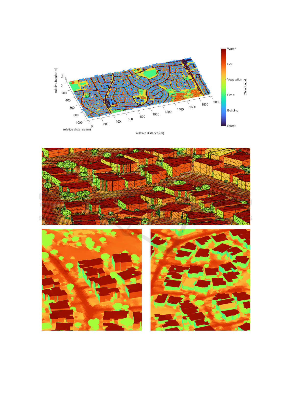
Figure 3: Reconstructed area as triangle mesh with respective class labels.

Figure 4: Qualitative results of the heat simulation on the LOD1 reconstruction of the urban area at 8pm. Top: simulated

surface temperatures displayed together with the triangle mesh. Bottom: simulated surface temperatures displayed without

triangle mesh. Left: view from the west. Right: view from the east.

GRAPP 2024 - 19th International Conference on Computer Graphics Theory and Applications

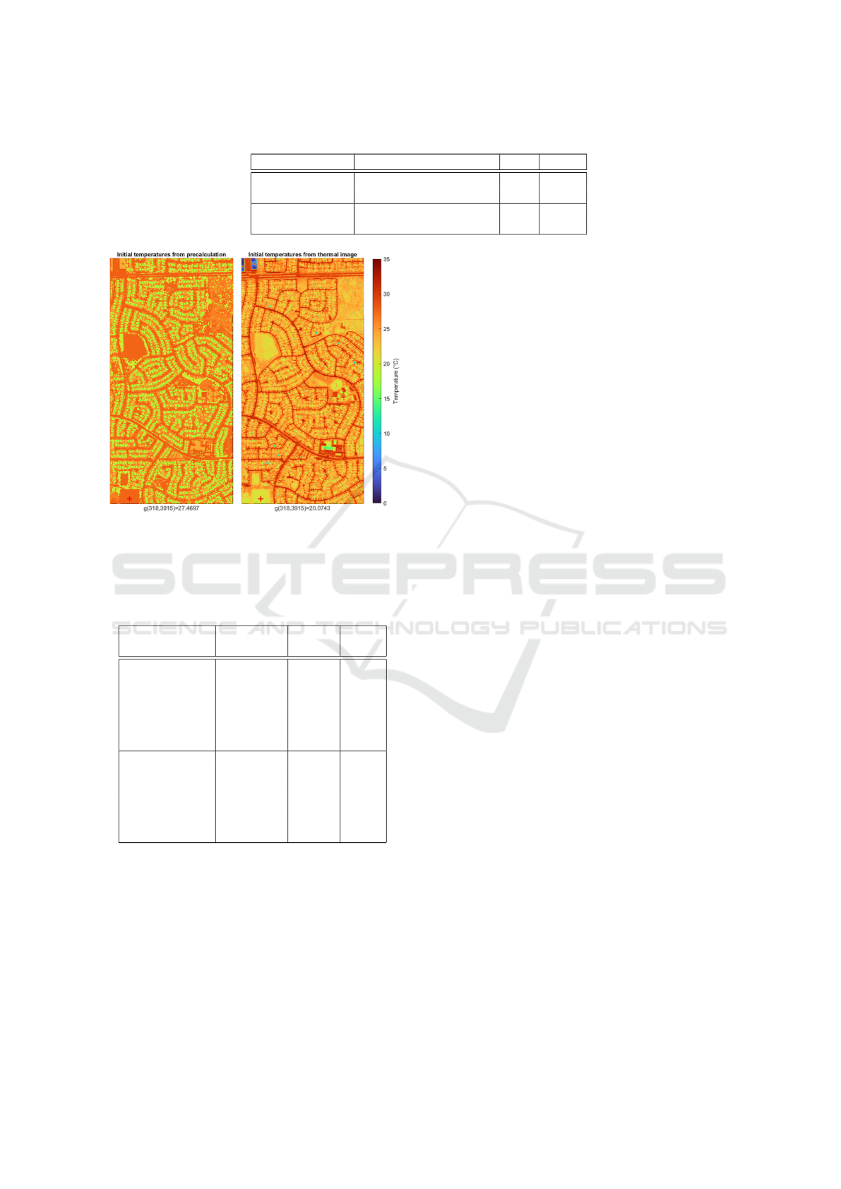
Table 1: Image similarity by mutual information (MI) and structural similarity index measure (SSIM).

Initial Condition Rendered Value MI SSIM

Precalculated Temperature 0.61 0.50

Long-Wave IR Radiance 0.60 0.63

Thermal Image Temperature 1.19 0.67

Long-Wave IR Radiance 1.00 0.67

Figure 5: Initial temperatures from precalculation (left), i.e.

material-dependent temperature value, and initial tempera-

tures from a given thermal image (right).

Table 2: Root-Mean-Square-Error (RMSE) and Mean Av-

erage Error (MAE) of simulated temperature values over all

classes, i.e. considering the full scene, and class-wise only.

Initial

Class RMSE MAE

Condition

Precalculated

All 8.56 6.96

Street 4.31 0.62

Soil 3.96 1.12

Gras 10.23 1.25

Buildings 13.58 12.96

Vegetation 5.52 5.40

Thermal Image

All 8.28 6.64

Street 4.34 0.73

Soil 2.98 0.89

Gras 7.85 0.97

Buildings 13.97 13.26

Vegetation 5.52 5.40

and radiances is applied. The resulting images, to-

gether with the measured aerial image, are displayed

in Figure 6. There, the effect of emissivity, i.e. the

material-dependent ability of surfaces to radiate heat,

can clearly be seen in the simulated long-wave in-

frared image. Simulation of the surface temperatures

took approximately 2 hours (application of initial

temperatures excluded) on a personal computer (In-

tel(R) Core(TM) i9-10900K, CPU@3.70GHz, 32GB

RAM, Nvidia GeForce RTX 2080 Super) and the

Matlab Parallelization Toolbox was used for GPU us-

age. Please note that the implementation of the math-

ematical model was conducted under the premise

of prototyping a simulation framework in an object-

orienting programming (OOP) matter in MATLAB

2021 and is not runtime-optimized. Therefore, ab-

solute run-times of the overall simulation are not rep-

resentative since OOP does not perform fast in MAT-

LAB, however, the ﬁnal coding structure of our im-

plementation is easily transferable to other program-

ming languages, allowing the fast implementation of

plugins for software in the ﬁeld of 3D graphics or vir-

tual environments.

As ﬁrst part of the evaluation, image similarity is

considered, and MI and SSIM are summarized in Ta-

ble 1. By determining the initial temperatures by the

given thermal image, MI is strongly increased. This is

expected and likely caused by the inner-class temper-

ature variations introduced by the initial temperatures.

Yet, MI is reduced when long-wave infrared radiance

is compared to the measured thermal image. Two po-

tential causes occur: ﬁrst, the radiance model might

be oversimpliﬁed. Second, the processing of the ther-

mal image before delivery causes unexpected and un-

documented deviations. The SSIM shows generally

good agreement between measurement and simula-

tion, yet, usage of long-wave infrared radiance instead

of surface temperatures shows none or only minor im-

provement, presumably for the same reasons as stated

above.

As second part of the evaluation, RMSE and MAE

of the simulated surface temperatures are determined

against the measured temperatures from the thermal

image, as previously outlined, and summarized in Ta-

ble 2. With an MAE of 6.96 for precalculated initial

values and 6.64 when the thermal image is applied

as initial condition, the need for a class-wise consid-

eration is raised. There, ground classes (street, soil,

gras) show good agreement with the measurements,

however, buildings and vegetation deviate, increasing

the comprehensive MAE. With vegetation being chal-

lenging to model due to its active nature, and given the

applied simpliﬁed model, a larger deviation than other

classes was expected. The high MAE value on build-

ings lies in an overestimation of roof temperatures,

cp. Figure 6, originating most likely from an underes-

timation of weather conditions and heavy generaliza-

Between Gaming and Microclimate Simulations: Temperature Estimation of an Urban Area

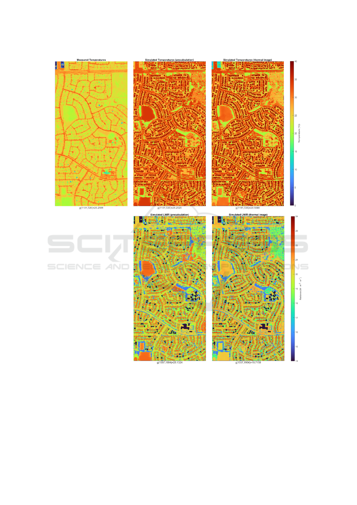
Figure 6: Measured and simulated thermal images. From left to right: measured temperatures from aerial thermal image,

simulated surface temperatures with initial temperatures from precalculation (top) with corresponding simulated long-wave

infrared radiance image (bottom), and simulated temperatures with initial temperatures from thermal image (top) with corre-

sponding simulated long-wave infrared radiance image (bottom).

GRAPP 2024 - 19th International Conference on Computer Graphics Theory and Applications

tions in roof construction. The underlying roof model

including insulation is generalized to most cities, yet

in our test area, i.e. the City of Melville, insulation is

often missing. Indeed, many buildings even allow for

air circulation between building walls and roof.

Comparing the initial conditions, only slightly

better results are found when the thermal image is

used. The precalculation is supposed to overcome the

thermal inertia rendering the initial condition crucial,

thus this minor improvement aligns with expected be-

havior. From the class-wise approach, ground sur-

faces suffer from outliers with large deviations be-

tween simulation and measurement. A reasonable ex-

planation are the neglected variations in moist, soil

composition, and street types (e.g. asphalt, concrete,

pavement).

In summary, the simulation shows good agree-

ment with the measured temperatures for most

classes, yet buildings and vegetation will need further

improvement in future work.

4 CONCLUSION

We presented a tool for temperature computation of

urban areas being more precise in thermal modeling

than game-oriented software yet less computation-

ally heavy than microclimate simulations. Starting at

meshes derived from multi-source sensor data, we are

driven by the motivation to create realistic tempera-

ture values which will allows for faster decisions in

urban planning.

We realized that the path from raw multi-source

sensor data to thermal image of an urban area is chal-

lenging and complex. The geo-referenced 3D para-

metric model, enriched with the weather data, makes

it possible to derive the temperatures of the scene

elements at any moment of time, and from there,

the radiance (infrared) image can be generated. The

negative consequence of a complex procedure is al-

ways that an inaccuracy at a very early stage re-

sults in barely inexplicable deviation from the refer-

ence data in the ﬁnal output. Providing a better co-

registration of sensor data; more robust procedures for

land cover and material classiﬁcation; higher levels of

details for buildings and trees; consideration of fur-

ther terms for infrared image synthesis out of surface

temperatures: all this inﬂuences the quantitative result

greatly. In this work, we concentrated on the under-

lying physics-based thermal models. Semantic- and

material-dependent models for conductive and con-

vective heat were presented. There, the convective

model by (Awol et al., 2020) has been adapted to real

urban areas. To handle the thermal inertia and the

challenging initial temperature conditions, material-

wise precalculation and usage of thermal imagery

were introduced, and the precalculation show promis-

ing results which is of importance as acquisition of

thermal imagery can be challenging.

In summary, our approach yielded promising re-

sults for a quick, superﬁcial screening of a large ur-

ban scene. Such a quick screening can assist in urban

planning. Yet, the simpliﬁed vegetation model of the

simulator at its current stage is a major drawback. Im-

proving this model, by integrating latent heat, is one

important direction of future work. Furthermore, we

strive for the inclusion of a simpliﬁed CFD simula-

tion, i.e. replacing the global wind velocity and direc-

tion by triangle-wise values. Naturally, as the current

implementation is in form of a prototype, we further-

more strive for a ﬁnal implementation and compari-

son of absolute runtimes to microclimate simulation

and gaming approaches.

ACKNOWLEDGEMENTS

Many thanks for providing the multi-source data of

the test site, City of Melville, particularly to Dr. Petra

Helmholtz from Curtin University, Australia.

REFERENCES

Awol, A., Bitsuamlak, G. T., and Tariku, F. (2020). Numer-

ical estimation of the external convective heat trans-

fer coefﬁcient for buildings in an urban-like setting.

Building and Environment, 169:106557.

Bartos, B. and Stein, K. (2015). FTOM-2D: a two-

dimensional approach to model the detailed thermal

behavior of nonplanar surfaces. In Stein, K. U. and

Schleijpen, R. H. M. A., editors, Target and Back-

ground Signatures, SPIE Proceedings, page 96530G.

SPIE.

Bulatov, D., Burkard, E., Ilehag, R., Kottler, B., and

Helmholz, P. (2020). From multi-sensor aerial data to

thermal and infrared simulation of semantic 3D mod-

els: Towards identiﬁcation of urban heat islands. In-

frared Physics & Technology, 105:103233.

Energie und Umwelttechnik (2009). W

arme- und

alteschutz von betriebstechnischen Anlagen in der

Industrie und in der technischen Geb

audeausr

ustung

- Berechnungsgrundlagen [Thermal insulation of

heated and refrigerated operational installations in

the industry and the building services - calculation

rules]. Technical Report VDI 2055 Blatt 1, VDI

Verein Deutscher Ingenieure e.V.

Kibler, C. L., Trugman, A. T., Roberts, D. A., Still, C. J.,

Scott, R. L., Caylor, K. K., Stella, J. C., and Singer,

M. B. (2023). Evapotranspiration regulates leaf tem-

Between Gaming and Microclimate Simulations: Temperature Estimation of an Urban Area

perature and respiration in dryland vegetation. Agri-

cultural and Forest Meteorology, 339:109560.

Kottler, B., Burkard, E., Bulatov, D., and Harak

e, L. (2019).

Physically-based thermal simulation of large scenes

for infrared imaging. In VISIGRAPP (1: GRAPP),

pages 53–64.

Liu, Z., Cheng, W., Jim, C. Y., Morakinyo, T. E., Shi, Y.,

and Ng, E. (2021). Heat mitigation beneﬁts of urban

green and blue infrastructures: A systematic review

of modeling techniques, validation and scenario sim-

ulation in ENVI-met V4. Building and Environment,

200:107939.

Oktal-SE (2023). Oktal Synthetic Environment.

http://www.oktal-se.fr/website/. Accessed: 2023-10-

26.

Presagis (2023). Presagis Canada Inc.

https://www.presagis.com/en/. Accessed: 2023-

10-26.

Rodr

ıguez-V

azquez, Martin and Hern

andez-P

erez, Iv

and Xam

an, Jesus and Ch

avez, Yvonne and Gij

on-

Rivera, Miguel and Belman-Flores, Juan M. (2020).

Coupling building energy simulation and computa-

tional ﬂuid dynamics: An overview. Journal of Build-

ing Physics, 44(2):137–180.

Ruijun Zhang, P. A. M. (2021). Cfd-cfd coupling: A novel

method to develop a fast urban microclimate model.

Journal of Building Physics, 44(5):385–408.

Wallrabe, A. (2001). Nachtsichttechnik: Infrarot-Sensorik:

physikalische Grundlagen, Aufbau, Konstruktion und

Anwendung von W

armebildger

aten [Low-light-level

technology: Infrared Sensor Technology: physi-

cal basics, structure, construction and application

of thermal imaging devices]. Springer, Braun-

schweig/Wiesbaden, 1st edition.

GRAPP 2024 - 19th International Conference on Computer Graphics Theory and Applications