
A Reinforcement Learning Environment for Directed Quantum Circuit
Synthesis
Michael K
¨
olle, Tom Schubert, Philipp Altmann, Maximilian Zorn, Jonas Stein
and Claudia Linnhoff-Popien
Institute of Informatics, LMU Munich, Munich, Germany
fi
Keywords:
Reinforcement Learning, Quantum Computing, Quantum Circuit Synthesis.
Abstract:
With recent advancements in quantum computing technology, optimizing quantum circuits and ensuring reli-
able quantum state preparation have become increasingly vital. Traditional methods often demand extensive
expertise and manual calculations, posing challenges as quantum circuits grow in qubit- and gate-count. There-
fore, harnessing machine learning techniques to handle the growing variety of gate-to-qubit combinations is
a promising approach. In this work, we introduce a comprehensive reinforcement learning environment for
quantum circuit synthesis, where circuits are constructed utilizing gates from the the Clifford+T gate set to
prepare specific target states. Our experiments focus on exploring the relationship between the depth of synthe-
sized quantum circuits and the circuit depths used for target initialization, as well as qubit count. We organize
the environment configurations into multiple evaluation levels and include a range of well-known quantum
states for benchmarking purposes. We also lay baselines for evaluating the environment using Proximal Pol-
icy Optimization. By applying the trained agents to benchmark tests, we demonstrated their ability to reliably
design minimal quantum circuits for a selection of 2-qubit Bell states.
1 INTRODUCTION
The field of quantum computing, including quantum
sensing, quantum meteorology, quantum communi-
cation, and quantum cryptography is recently receiv-
ing a lot of attention (T
´
oth and Apellaniz, 2014; Ek-
ert, 1991). Consequently, directed quantum circuit
synthesis (DQCS) involving quantum state prepara-
tion, which plays a vital role in the above-mentioned
technologies, gains more and more interest. Current
quantum circuit layouts range from rather straightfor-
ward ones, as used for Bell state preparation (Barenco
et al., 1995; Bennett and Wiesner, 1992; Nielsen
and Chuang, 2010), to highly sophisticated designs
including tunable parameters, as present in Varia-
tional Quantum Classifiers and Variational Quantum
Eigensolvers (Farhi and Neven, 2018; Schuld et al.,
2020; Peruzzo et al., 2013). Though many approaches
addressing quantum circuit development are known,
most of them focus on the optimization of already
existing circuits (F
¨
osel et al., 2021; Li et al., 2023).
On the contrary, research regarding the circuit syn-
thesis is sparse, making manual methods still a state-
of-the-art technique for tackling these tasks. This cir-
cumstance gets especially problematic if the involved
quantum circuits increase in qubit number and gate
count, resulting in large state-spaces with an expo-
nential amount of possible layouts. Hence, to guar-
antee efficient task-solving, it is crucial to develop an
approach that tackles the problem of DQCS and de-
creases the amount of required human insight.
On consideration of the aforementioned examples,
it becomes apparent that machine learning (ML) ap-
proaches are especially suited for subjects involving
complex calculations and elaborate combinatorial op-
timizations. Hence, we consider a ML-based tech-
nique for the DQCS problem. Since quantum circuit
construction and optimization does not entail learn-
ing from data in the classical ML sense, we instead
apply the concept of improving by repeated interac-
tion with a problem environment via reinforcement
learning (RL). While research for applying RL on
state preparation tasks is known, there is limited ex-
ploration of the underlying DQCS problem and the
implementation on actual quantum hardware utilizing
a set of distinct quantum gates (cf. (Gabor et al., 2022;
Mackeprang et al., 2019)). Similarly, the disassembly
of a proposed circuit into a sequence of valid quantum
gates is a crucial step in facilitating the transfer to a
real quantum device (Mansky et al., 2022).
Kölle, M., Schubert, T., Altmann, P., Zorn, M., Stein, J. and Linnhoff-Popien, C.
A Reinforcement Learning Environment for Directed Quantum Circuit Synthesis.
DOI: 10.5220/0012383200003636
Paper published under CC license (CC BY-NC-ND 4.0)
In Proceedings of the 16th International Conference on Agents and Artificial Intelligence (ICAART 2024) - Volume 1, pages 83-94
ISBN: 978-989-758-680-4; ISSN: 2184-433X
Proceedings Copyright © 2024 by SCITEPRESS – Science and Technology Publications, Lda.
83

We introduce the Quantum Circuit RL environ-
ment designed to train RL agents on the task of
preparing randomly generated quantum states uti-
lizing the Clifford+T gate set, enabling the trained
agents solve the DQCS problem for arbitrary target
states. In our environment, we view the use of quan-
tum gates on quantum states as actions and the quan-
tum state as observation. The objective is to prepare
a specific target state efficiently, and success is mea-
sured by minimizing the number of gates needed to
construct the quantum circuit. We also evaluate Prox-
imal Policy Optimization algorithm agents on differ-
ent configurations of our environment to form a base-
line. Lastly, we benchmark the trained agents on a set
of well-known 2-qubit states.
This work is structured as follows. We first give a
short overview of the related work in Section 2. We
then introduce our Quantum Circuit Environment for
circuit synthesis in Section 3, followed by our experi-
mental setup in Section 4 and results in Section 6. Fi-
nally, we conclude with a summary and future work
in Section 7.
2 RELATED WORK
In this section we introduce underlying concepts es-
sential for a clear comprehension of our research.
Further we provide an overview of prior work in the
field of AI-assisted quantum circuit generation and
optimization, connecting it to our approach.
2.1 Quantum States
Quantum computing is an emerging technology dis-
tinguishing itself from classical computing funda-
mentally by the usage of so-called quantum bits or
qubits instead of classical bits as units of information
storage. Qubits among other aspects differ from their
classical counterparts by showing the ability of super-
position. This describes the ability of the qubit to not
only be in one of the discrete states 0 or 1, like a clas-
sical bit, but to be in any linear combination of 0 and
1, enlarging the available state-space from discrete to
continuous. Eq. 1 defines the quantum state of one
qubit in Dirac- and vector-notation.
|
q
⟩
= α
|
0
⟩
+ β
|
1
⟩
=
α
β
α, β ∈ C (1)
Another characteristic of qubits is the so-called entan-
glement, which describes the possibility of correlat-
ing the states of multiple qubits, enabling the setup of
complex relations between them. Another option for
the description of quantum states is the density matrix
representation given in Eq. 2.
ρ =
|
q
⟩⟨
q
|
=
|α|
2
αβ
∗
α
∗
β |β|
2
α, β ∈ C (2)
To compare two density matrices and hence two quan-
tum states ρ and
e
ρ, the fidelity F as given in Eq. 3 is
used as a measure.
F(ρ,
e
ρ) =
tr
q
√
ρ
e
ρ
√
ρ
2
(3)
When solely states in vector representation are con-
sidered, this equation simplifies to the expression
given in Eq. 4(Jozsa, 1994).
F(ρ,
e
ρ) = |
⟨
q
||
e
q
⟩
|
2
(4)
2.2 Quantum Circuits
Quantum computers use logic gates, represented by
unitary matrices denoted as U, to transform a quan-
tum state
|
Φ
⟩
into a new state
|
Φ
′
⟩
following Eq. 5.
Φ
′
= U
|
Φ
⟩
(5)
The unitarity aspect of the gates makes all operations
relying on these gates unitary and hence reversible. A
generic unitary matrix working as a quantum mechan-
ical operator on a single qubit can be defined accord-
ing to Eq. 6.
U = e
i
γ
2
cosθe
iρ
sinθe
iφ
−sinθe
−iφ
cosθe
−iρ
(6)
In the unitary matrix U, γ denotes a global phase mul-
tiplier, θ characterizes the rotation between compu-
tational basis states, while ρ and φ introduce relative
phase shifts to the diagonal and off-diagonal elements
respectively. Different quantum gates can be created
by selecting specific values for the involved parame-
ters. By leaving some of the involved parameters un-
defined, the design of parameterized quantum gates is
possible. Another characteristic of a quantum gate is
its multiplicity, defining the number of qubits the gate
acts on. Several different gates can then be combined
within a gate set (e.g. the strictly universal Clifford+T
gate set given in Table 1).
A quantum circuit is then formed by a sequence of
quantum gates acting upon a number of qubits, while
the overall number of gates within the quantum circuit
is called the circuit-depth. Hence the circuit repre-
sents one big transformation matrix, transforming the
incoming quantum state provided by the input qubits
into an altered quantum state obtained on the output
qubits.
ICAART 2024 - 16th International Conference on Agents and Artificial Intelligence
84
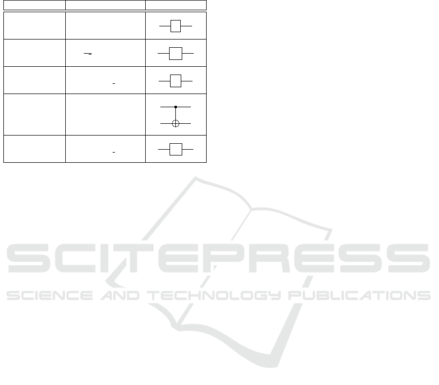
Table 1: The gates in the Clifford+T gate set, along with
their corresponding matrix representations and circuit sym-
bols. For the CNOT gate, the example provided illustrates
the scenario where the first qubit acts as the control bit.
Symbol (Name) Matrix representation Circuit notation
I (Identity)
1 0
0 1
I
H (Hadamard)
1
√
2
1 1
1 −1
H
S
1 0
0 e
i
π
2
S
CNOT
1 0 0 0
0 1 0 0
0 0 0 1
0 0 1 0
T
1 0
0 e
i
π
4
T
2.3 Quantum State Preparation
Recently much effort has gone into the investigation
of quantum state preparation for different quantum-
based fields like quantum meteorology, quantum
sensing, quantum communication, and quantum com-
puting to name just a few examples (Krenn et al.,
2015; Krenn et al., 2021; Mackeprang et al.,
2019). Further exploiting computational resources,
approaches facilitating state preparation using ML
methods were done Mackeprang et al. investigated
the state preparation of 2-qubit quantum states using
RL algorithms showing their ability to generate Bell
states finding the same solutions as previously dis-
covered by humans (Mackeprang et al., 2019; Zhang
et al., 2019).
A different approach towards automated quantum
state preparation was investigated by Gabor et al. (Ga-
bor et al., 2022). Their study involved an approach
training an RL agent to generate quadratic transfor-
mation matrices transforming a initial state into a tar-
get state, both given in the density matrix representa-
tion. To account for unitarity of the transformation,
they utilized a QR-decomposition disassembling the
initially obtained matrix A according to A = U ·R,
while U represents a unitary and R an upper trian-
gular matrix. Subsequently, they used U as the uni-
tary transformation matrix. With this technique they
reached state fidelities of up to > 0.99 for individual
target-states, but struggled with arbitrary state prepa-
ration, resulting in unrealistically long circuits (even
on small 2 qubit circuits) (Gabor et al., 2022).
Their research showed a promising way to ap-
proach the subject of quantum state preparation open-
ing up new possibilities, but also pointed out sev-
eral difficulties. The studies done in this project are
closely connected and partially based on the research
of Gabor et al., dealing with a similar kind of state
preparation problem, while focusing on the possible
improvements in the following. One issue of the ap-
proach chosen by Gabor et al. might be the con-
struction of potentially non-unitary quadratic matri-
ces, leading to costly QR-decomposition scaling with
a complexity between O(n
2
) and O(n
3
), if n is the di-
mension of the quadratic matrix (Parlett, 2000). To
improve this approach, we exclusively utilize unitary
transformations as provided by the Clifford+T gate
set, reducing computational demands and accelerat-
ing agent learning. To simplify the approach used by
Gabor et al. we substituted the density matrix rep-
resentation by a vector representation, reducing the
dimensions of the representation from N
2
to N poten-
tially lowering the computational costs.
2.4 Quantum Circuit Optimization and
Synthesis
Since manual optimization is a time-consuming,
error-prone process requiring a high amount of
knowledge, automation of quantum circuit synthe-
sis and optimization is crucial (F
¨
osel et al., 2021).
Consequently, there is a rising focus on employ-
ing machine learning algorithms to tackle this chal-
lenge (Cerezo et al., 2021; Pirhooshyaran and Terlaky,
2021; Ostaszewski et al., 2021; Altmann et al., 2023).
An approach from F
¨
osel et al. aims to optimize arbi-
trary generated quantum circuits with regards to their
complexity using a CNN approach, yielding an over-
all depth and gate reduction of 27% and 15% respec-
tively (F
¨
osel et al., 2021). Further Zikun et al. im-
plemented an RL-based procedure utilizing a graph-
based framework to represent the structure of a certain
quantum circuit. Their proposed algorithm (QUARL)
then optimizes the respective circuit with regard to its
gate count, while maintaining its overall functional-
ity achieving a gate reduction ranging around 30%.
However, most of the approaches focus on the opti-
mization of already existing circuits disregarding their
initial synthesis. To address this issue, our study in-
cludes the initial quantum circuit synthesis into the
procedure (Li et al., 2023; Xu et al., 2022).
3 QUANTUM CIRCUIT
ENVIRONMENT
In this section, we introduce a versatile and scal-
able reinforcement learning environment designed for
A Reinforcement Learning Environment for Directed Quantum Circuit Synthesis
85

quantum circuit synthesis. This environment estab-
lishes a foundational platform for researchers to em-
ploy machine learning in discovering new and effi-
cient quantum circuits for known problems. At each
step, a RL agent can place one quantum gate onto a
circuit, with the aim of crafting a circuit that maps
from an arbitrary initial state to an arbitrary target
state. We formulate the problem at hand as a Markov
decision process M = ⟨S, Γ, P , R, γ⟩ where S is a set
of states s
t
at time step t, Γ is a set of actions a
t
,
P (s
t+1
|s
t
, a
t
) is the transition probability from s
t
to
s
t+1
when executing a
t
, r
t
= R(s
t
, a
t
) is a scalar re-
ward, and γ ∈ [0, 1) is the discount factor (Puterman,
2014). For our implementation, we use the Penny-
lane framework to efficiently simulate quantum cir-
cuits. The project is open-source
1
, distributed under
the MIT license and available as a package on PyPI.
In the following sections we elaborate on the details
of the Quantum-Circuit environment.
3.1 Observation Space
We define an observation in our environment as a real
vector of length 2
n+2
. Since a normalized n-qubit
quantum system can be expressed as a complex vector
in 2
n
dimensions, we start with two complex vectors
describing the current quantum state (v) and the de-
sired target quantum state (ˆv), each of length 2
n
.
v =
v
1
v
2
·
·
·
v
2
n
∩ ˆv =
ˆv
1
ˆv
2
·
·
·
ˆv
2
n
⇒ s =
Re(v
1
)
Re(v
2
)
.
.
.
Re(v
2
n
)
Im(v
1
)
Im(v
2
)
.
.
.
Im(v
2
n
)
Re( ˆv
1
)
Re( ˆv
2
)
.
.
.
Re( ˆv
2
n
)
Im( ˆv
1
)
Im( ˆv
2
)
.
.
.
Im( ˆv
2
n
)
∀
i∈{1··2
n
}
v
i
, ˆv
i
∈ C ∩ s ∈S
(7)
The concatenation of both results in a complex
vector of length 2
n+1
. Splitting up the complex coef-
ficients of the resulting vector into the real and imag-
inary part we end up with the 2
n+2
real dimensions
characterizing the vector s in observation-space S.
1
https://github.com/michaelkoelle/rl-qc-syn
With the current state (v) included in s describing the
complete state of the quantum system, the environ-
ment is fully observable. Further the observation con-
tains the desired target state ( ˆv) to maintain a consis-
tent target perspective for the RL agent.
3.2 Action Space
The action space Γ is multi-discrete and defined by
two finite sets of a specific size, out of which one el-
ement is drawn respectively to form an action. While
one set accounts for all gates included in the input
gate set G, the other set represents all possible com-
binations of qubits inputted into the respective gate,
given a total number of n qubits. Eq. 8 calculates the
size of the action-space with regards to the given G
and n, with n
max
being the number of qubits taken
by the gate g ∈ G processing the highest number of
qubits within the gate set.
Γ = [{0, 1.., |G|}, {0, 1..,C}]
with C =
n!
(n −n
max
)!
(8)
A proper mapping between the integers in the action-
space and the corresponding gate-qubit combination
is achieved in two steps. The first value serves as an
index for a list representing the gate set, thus selecting
a specific gate. The second value indexes a listing of
all qubit permutations possible, given distinct values
for n and n
max
. Through this, it is decided which qubit
combination the selected gate is applied on. In case
the gate takes fewer qubits than present in the respec-
tive combination, the gate is simply applied on the
first n
g
qubits of the permutation, while n
g
represents
the number of qubits taken by the gate. Implementing
the action space using the two-set architecture ensures
that in a random sampling case, the selection of every
gate and every combination is equally probable. On
the contrary, utilizing just one set including all possi-
ble gate-qubit combinations in the first place, would
lead to an unequal weighting of gate selection. This
happens since gates taking a higher qubit number than
others are applicable to a larger number of different
qubit combinations and thus would appear more often
in the set. Hence we chose the two-set architecture.
3.3 Reward
The quantum circuit environment comes with two dif-
ferent reward functions that are user selectable, a step-
penalty reward (Eq. 9) and a distance-based reward
(Eq. 10).
ICAART 2024 - 16th International Conference on Agents and Artificial Intelligence
86
r
1
=
(
L −l −1 if 1 −F < SFE
−1 otherwise
(9)
Note that l refers to the depth of the current quan-
tum circuit, L is the maximum circuit depth before
terminating the episode, F references the fidelity from
Eq. 3 and SFE is the standard fidelity error describing
the deviation of the fidelity F from the value 1.
r
2
=
L −l −1 if 1 −F < SFE
−⌊
L
2
⌋·(1 −F) if 1 −F ≥ SFE ∧ l = 0
−1 otherwise
(10)
When comparing both equations, it becomes obvious
that they are equivalent apart from the case when the
episodes are finished without reaching the target. In
the step-penalty reward equation, the agent just re-
ceives another −1 penalty, whereas in the distance re-
ward equation, the final penalty is proportional to the
distance of the current state to the target state (1−F).
Using this approach, the agent receives additional in-
formation about the closeness to the target, even if it
was not able to reach it completely. This additional
information may foster the learning procedure of the
agent, especially when more complex targets are in-
volved.
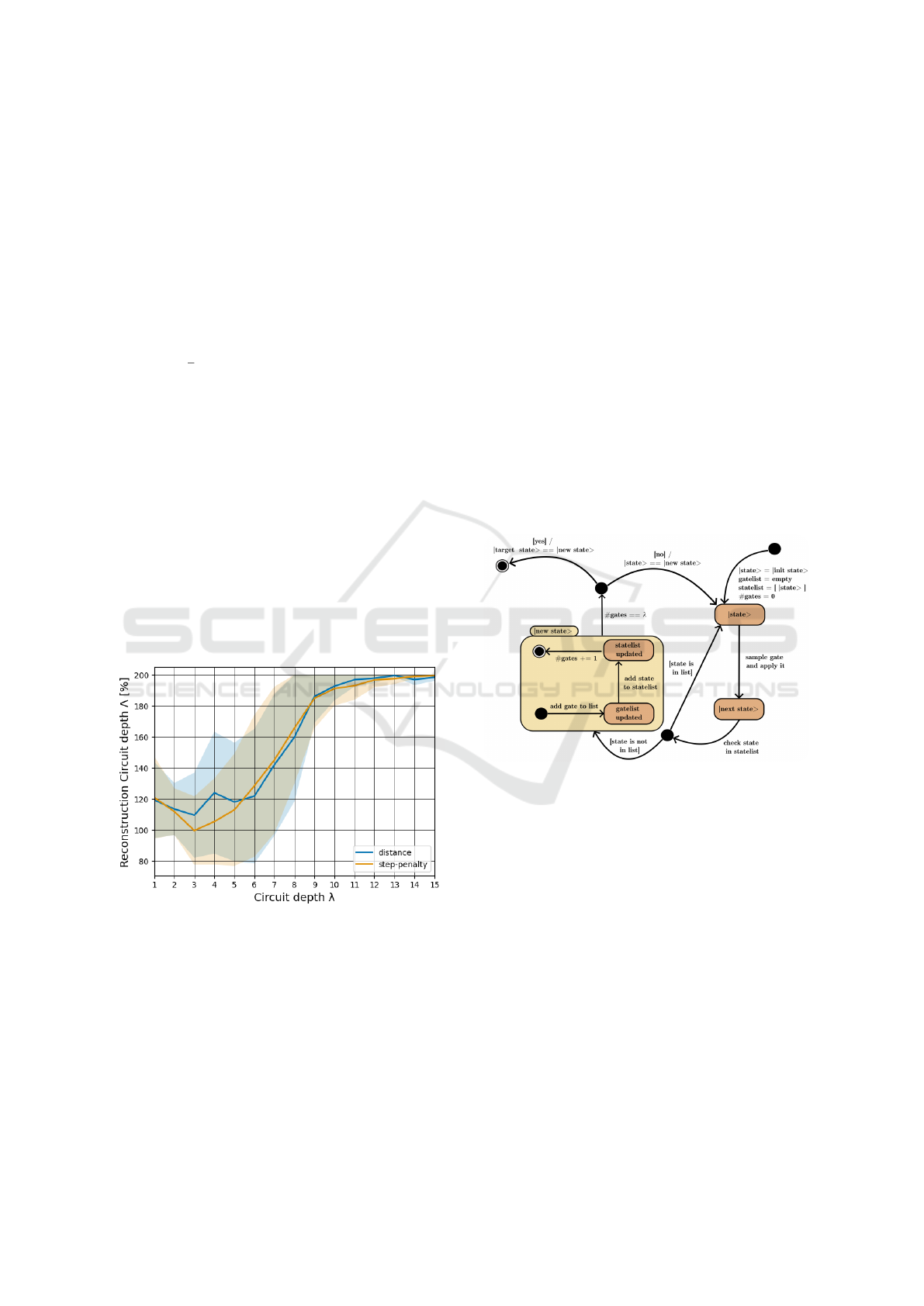
Figure 1: Comparison of two reward techniques: step-
penalty and distance. Each data point represents the average
performance of three runs, trained in a 2-qubit environment
with varied target circuit-depth.
We evaluated both reward functions on 2-qubit-
systems with targets characterized by circuit-depths λ
from 1 to 15, following the target-initialization algo-
rithm (see Section 3.4). We executed 3 runs for ev-
ery setting. Data points were obtained by averaging
the reconstruction circuit-depth Λ (see Section 4.2)
over the last 100 training episodes, with each agent
undergoing identical training steps. Analysis of the
reward technique comparison in Fig. 1 reveals that
while step-penalty and distance rewards exhibit sim-
ilar behaviors, key differences emerge. Specifically,
the step-penalty curve appears smoother and demon-
strates a higher quality, correlating to a 5-20% reduc-
tion in reconstructed circuit-depths Λ at lower λ ∈
{2, 3,4, 5}. Owing to its robust performance and sta-
bility, especially at lower difficulty targets, the step-
penalty technique was adopted as standard for all sub-
sequent experiments.
3.4 Target State Initialization
When initializing the environment, either a target
quantum state or a circuit-depth λ must be specified.
If a target quantum state is set, a maximum depth
L must also be defined, upon exceeding the current
episode will terminate. We included this option to
provide the possibility to apply agents on specific,
fixed target states.
Figure 2: State diagram displaying the target state gen-
eration algorithm, while gate-list and state-list are imple-
mented as actual lists and λ is the circuit-depth parameter
defining the absolute number of gates, which must be ap-
plied to get to the target. The algorithm starts at the upper
right side of the figure.
If no target parameter is provided, the circuit-
depth parameter λ must be set, enabling the gener-
ation of a random target state per episode, as illus-
trated in Fig. 2. The parameter λ denotes the neces-
sary quantum gate count, applied via a defined algo-
rithm, to reach the target state. To ensure each gate
meaningfully alters the circuit, a change condition is
enforced for every additional gate, permitting its ap-
plication only if the state change satisfies the condi-
tion 1 −F ≥ 0.001, with F corresponding to the fi-
delity. The change condition is then determined be-
tween the state after gate application and every state
previously visited within the initialization procedure
A Reinforcement Learning Environment for Directed Quantum Circuit Synthesis
87

respectively. If one of the conditions is not satis-
fied then the gate is not applied. By this ineffective
or neutralizing gate applications are avoided. For in-
stance, with the Clifford+T gate set, redundancy can
arise due to the self-inverse nature of Hadamard- and
CNOT-gates. Utilizing this method mitigates cyclical
patterns during target initialization and enhances the
approximation accuracy of the actual minimal gate
count to the provided λ. However, exact equivalence
is not assured. If a permitted gate cannot be applied
after 2 ×|G| consecutive tries, where |G| signifies the
gate set cardinality, the generation process is reset to
prevent stagnation at a specific state.
3.5 Training Loop
Once the environment is initialized, the agent receives
the initial quantum state and target state as first ob-
servation in the format specified in Eq. 7. The agent
now chooses an action in the format specified in Eq. 8
based on the observation. This action corresponds to
a gate applied to a specific combination of qubits. The
environment appends the received action to the list of
previously taken actions. The updated list of actions is
then applied sequentially to form the respective quan-
tum circuit present at the current step. Running the
updated circuit then produces the succeeding obser-
vation equivalent to the next state of the environment.
Following this procedure starting from a specified ini-
tial state (e.g. |00...0⟩), the agent tries to apply a se-
quence of gates in order to get to the defined target
state. This process is displayed in Fig. 3. After the
Figure 3: Schematic of the sequential application of the up-
dated list of actions on the initial state |00..0 > transforming
it to the current state outputted by the environment.
application of the chosen gate, the number of steps
taken is increased by one, tracked by a step-counter
variable l. In case l reaches the maximal calculation
length L, the episode is aborted. L, if not defined at
the environments’ initialization together with a spe-
cific target state, is determined by the otherwise given
circuit-depth parameter λ according to Eq. 11.
L = 2 ·λ (11)
The other case in which the current episode is termi-
nated occurs when the target state is reached. Hence
one episode of the environment can be defined by tak-
ing steps starting from the initial state, either until the
target state is reached or until the number of already
taken steps equals the maximal calculation length L.
When the episode is terminated in case no target state
parameter is set, a new target is generated following
the algorithm described in Fig. 2 prior to the start of
the next episode. Additionally, the current state is re-
set to the initial state and the step counter variable l is
set to 0 when a new episode is started.
4 EXPERIMENTAL SETUP
In the following section we go into details about how
we set up our experiments. We explain our choice of
baseline algorithm and propose the reconstructed cir-
cuit depth as an evaluation metric specifically for the
quantum circuit environment. Lastly, we elaborate on
the training procedure and the used hyperparameters.
4.1 Baselines
In order to evaluate our environment designed for
quantum circuit synthesis, we conducted tests using
RL. Inspired by the approach of Gabor et al., we used
Proximal Policy Optimization (PPO) and Advantage
Actor-Critic (A2C) based agents as implemented in
the stable-baselines framework, while adding a ran-
dom agent for comparison reasons. Our aim was to
identify and select the highest-performing algorithm
among these, which was then utilized for our main
experiments.
Our primary baseline, the random agent, serves
as a rudimentary control, making arbitrary selections
from the action space. This agent applies quantum
gates onto the qubits without any informed guidance
or strategy, providing a baseline performance metric
which any proficient strategy should surpass.
Next, we implemented a PPO agent, which opti-
mizes the policy by constraining the new policy to be
close to the old policy (Schulman et al., 2017). After
performing a minor hyperparameter search, particu-
larly focusing on the learning rate, the agent was eval-
uated on a 2-qubit circuit with varying circuit depths
over three runs.
Likewise, A2C was evaluated, a synchronous,
deterministic variant of A3C which uses advantage
functions to reduce the variance of the policy gradient
estimate (Mnih et al., 2016). Following a similar ex-
perimental protocol as with PPO, it was subjected to
a limited hyperparameter search, primarily adjusting
the learning rate, and further evaluated under identical
conditions on the 2-qubit circuit.
PPO distinctly outperformed A2C in synthesizing
2-qubit circuits across varied circuit depths, manifest-
ing more consistent and proficient results over the
three runs. The evaluations were quantitatively as-
sessed based on the circuit-depth λ, ensuring a com-
ICAART 2024 - 16th International Conference on Agents and Artificial Intelligence
88

prehensive appraisal across numerous scenarios and
depths. Henceforth, due to its demonstrable superior-
ity in our preliminary experiments, PPO was selected
as the algorithm of choice for succeeding experiments
and evaluations throughout our research.
4.2 Reconstructed Circuit-Depth Metric
Establishing a performance metric is crucial to main-
tain a general comparability within the RL environ-
ment, particularly when involving diverse agents and
parameterizations. Comparing different runs with
varying configurations is difficult because the rewards
scale with the used parametrization. To address this,
we introduce the reconstructed circuit-depth metric,
designed to normalize rewards with respect to the
configuration, thereby facilitating a straightforward
comparison across runs and giving a much more clean
reading on the actual performance of the agent. By
normalizing the number of gates used by the agent
to recreate the target n
g
through circuit-depth λ used
for target initialization, a generally valid measure
can be designed. This metric then represents how
well the agent performed, normalized on the prede-
fined circuit-depth. Defining the maximal calculation
length L according to Eq. 11 and extracting the re-
maining calculation length of the current episode, n
g
can easily be derived using Eq. 12.
n
g
= L −l (12)
Following the intuitive setup of the general measure
mentioned above, we define a metric called the re-
constructed circuit-depth Λ via Eq. 13.
Λ[%] =
n
g
λ
·100% (13)
Achieving Λ = 100% signifies that the agent has
found a method to recreate the target with equal
circuit-depth as the initial generation algorithm. The
metric’s limit extends to 200%, considering that the
maximum n
g
value equals L. Consequently, recon-
structed circuit-depths ranging between 100% and
200% or below 100% indicate respectively longer or
shorter gate sequences found by the agent compared
to the intended gate sequence.
5 TRAINING AND
HYPERPARAMETER
OPTIMIZATION
To assure a robust and replicable training process,
each model configuration was trained under consis-
tent conditions on a Slurm cluster, utilizing Intel(R)
Core(TM) i5-4570 CPU @ 3.20GHz and Nvidia 2060
and 1050 GPUs, for a substantial total of 1,700,000
steps (56667 - 1700000 episodes, dependent on the
settings) per run. Three different seeds, namely
{1, 2,3}, were used for all experiments to obtain con-
sistent and reliable results, outputting an average and
a standard deviation for each data point. If not further
specified, we use a 2 qubit system with a circuit depth
of 5 and a SFE of 0.001. Furthermore, we use an ini-
tial state of |00...0 >, since it is the ground state of
most quantum hardware and thus a prominent start-
ing point (Schneider et al., 2022; Kaye et al., 2007;
Blazina et al., 2005).
A hyperparameter search was conducted,
focusing on the learning rate, using a grid
search approach across the following candidates:
0.00001, 0.0001,0.0003, 0.0005,0.0007, 0.001, 0.01.
For the Proximal Policy Optimization (PPO) al-
gorithm, a learning rate of 0.001 was identified as
optimal and was subsequently utilized in all related
experiments. Additionally, the clipping parameter
for PPO was set to 0.2 to ensure stable and reliable
policy updates. On the other hand, the Advantage
Actor-Critic (A2C) algorithm demonstrated optimal
performance with a learning rate of 0.00001.
This meticulous approach to training and hyper-
parameter optimization lays a solid foundation for
the subsequent experiments, ensuring that the derived
results and insights are both reliable and grounded
in a systematic exploration of the model’s parameter
space.
6 RESULTS
A main objective of our project was the implemen-
tation of a RL environment capable of training RL
agents on the DQCS problem. Another one was to
study the DQCS itself. Therefore, we now conduct
a variety of experiments to examine the task. For
the setup used in the following experiments, see Sec-
tion 4.
A comparison of PPO and A2C used with the re-
spective optimized settings showed a clear superior-
ity of the PPO algorithm. We evaluated the last 100
episodes of the respective runs of the agents on 2-
qubit targets with circuit-depth λ = 5. The recon-
structed circuit-depth Λ reached by the PPO agents
was 112.5±35.3%, while the A2C agents produced a
Λ of 195.3±6.5%. In comparison the random base-
line, corresponding to an untrained agent, exhibited a
Λ = 199.6 ±2.8%. Due to the better performance of
PPO it was selected for all following experiments.
A Reinforcement Learning Environment for Directed Quantum Circuit Synthesis
89
6.1 Qubit – Circuit-Depth Relationship
In order to explore the complexity of the DQCS prob-
lem, we investigated the training of PPO-agents on
various systems differing in their qubit numbers and
circuit-depths λ. We trained agents on systems of
2, 3, 4, 5, and 10 qubits utilizing circuits of depths
λ from 1 to 15 respectively. We obtained the data
displayed in Fig. 4 by averaging the reconstructed
circuit-depth Λ of the respective trained agents over
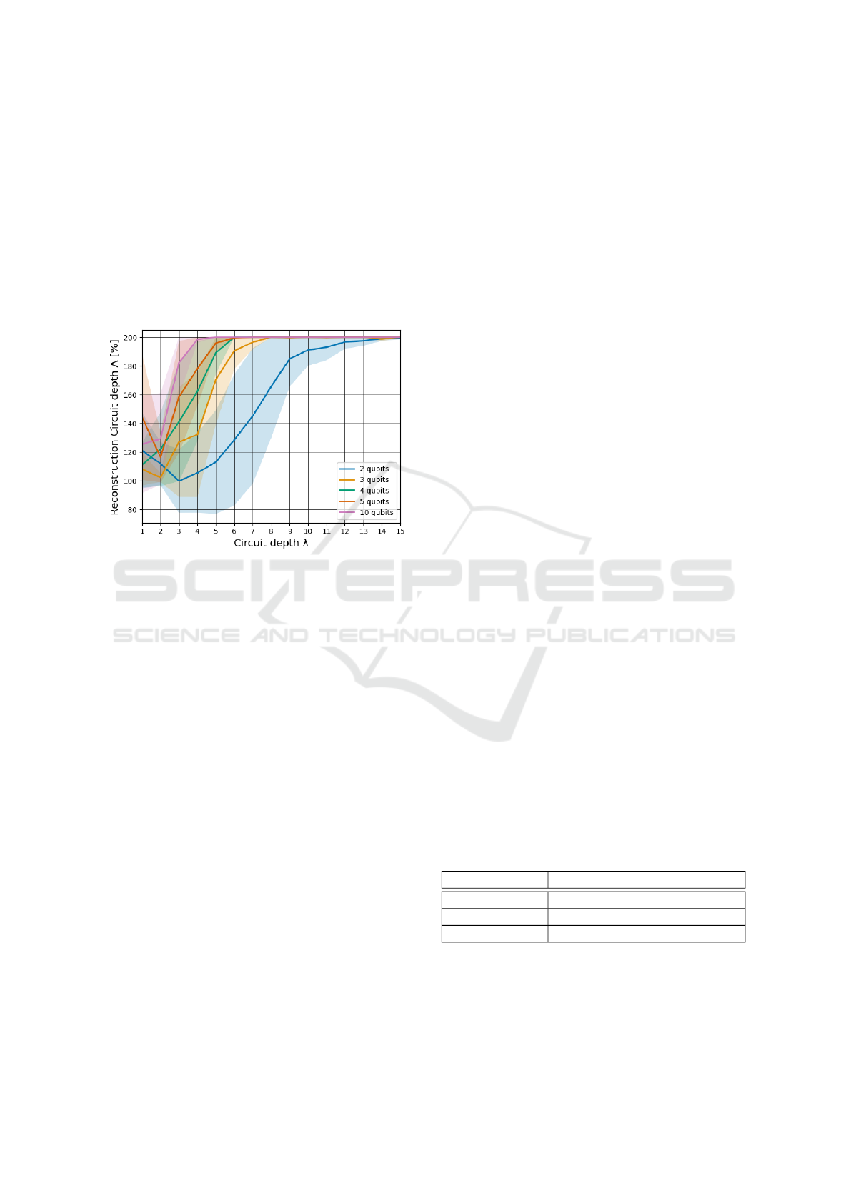
the last 100 episodes of the training run. Analyz-
Figure 4: Agents’ performances on targets with different
qubit numbers n (2, 3, 4, 5, 10) while the circuit-depth λ
is varied (1-15). Every data point represents the average
performance of 3 agents trained on systems possessing the
respective n and λ settings.
ing the curves, two main trends get apparent. The
first observed trend is the increasing reconstructed
circuit-depth (Λ) as the target circuit-depth (λ) rises,
resembling a sigmoid curve. A higher target circuit-
depth (λ) naturally demands more intricate solutions
from the agent for their preparation. Starting from the
left side of the plot, the reconstructed circuit-depth
(Λ) ranges from 100% to 140% indicating scenarios
where the agent’s solutions resemble the paths used
for target initialization. The curves exhibit a linear
rise before eventually asymptotically converging to-
wards a Λ of 200%. This indicates the agent’s inabil-
ity to recreate the target at this level of complexity.
The second trend involves a decrease in agent per-
formance as the qubit number (n) increases, reflect-
ing the increased complexity of the target state. This
is evident from the steeper rise in the reconstructed
circuit-depth (Λ) occurring at lower λ-values for tar-
gets with higher n compared to those with lower n. Of
particular interest is the situation at λ = 3 and n = 2
(represented by the blue curve), where the curve tan-
gentially intersects the 100% mark. This scenario
offers two possible explanations. First, it could im-
ply that the agent perfectly recreates every target us-
ing an equivalent circuit-depth as applied during ini-
tialization. Alternatively, it suggests that the agent
achieves the desired states with a lower circuit-depth
and, consequently, fewer quantum gates than initially
used to create the targets. Consequently, the aver-
age reconstruction circuit-depth (Λ) can reach 100%
or even drop below it. This observation, considering
the advanced algorithm used for target initialization,
provides evidence of the high level of optimization
achieved by the trained agents.
6.2 Benchmarking Analysis
In the following section, we set up a benchmarking
framework for the quality validation of the trained
agents and for the comparison of different RL algo-
rithms on the DQCS problem. We focus on the exam-
ination of comparatively simple systems for bench-
marking, involving 2-qubit targets only. To facilitate
the benchmarking, we conducted two different ap-
proaches. The first method measures the performance
of an agent on a set of randomly generated targets of a
certain circuit-depth λ, the other applies the agent on
a set of specific well-known target states.
6.2.1 Evaluation Levels
The difficulty of the target circuit is dependent on two
different factors, the number of qubits and the circuit-
depth λ used for target initialization. However, setting
the qubit number to 2 leaves us with λ as the only pa-
rameter. Based on the data obtained in Section 6.1,
we are able to propose a splitting of the parameter-
space of λ [1,15] into three evaluation levels ’easy’,
’medium’, and ’hard’. According to Fig. 4, the first
segment describes a development varying around a re-
constructed circuit-depth of 110%. The second region
can be defined as an interval of linear rise and the last
section is characterized by an asymptotic convergence
against a reconstructed circuit-depth of 200%. Table 2
contains the definition of the derived levels.
Table 2: The definition of the three evaluation levels ’easy’,
’medium’ and ’hard’ within the circuit-depth λ interval of
[1, 15].
Level Set of included circuit-depths λ
easy {1, 2, 3, 4, 5}
medium {6, 7, 8, 9, 10}
hard {11, 12, 13, 14, 15}
The data displayed in Fig. 5 was obtained by ap-
plying agents trained on 2-qubit targets with different
circuit-depths λ, ranging from 1 to 15 on 100 ran-
dom targets of the respective evaluation level, while
setting all other parameters to the standard values.
ICAART 2024 - 16th International Conference on Agents and Artificial Intelligence
90
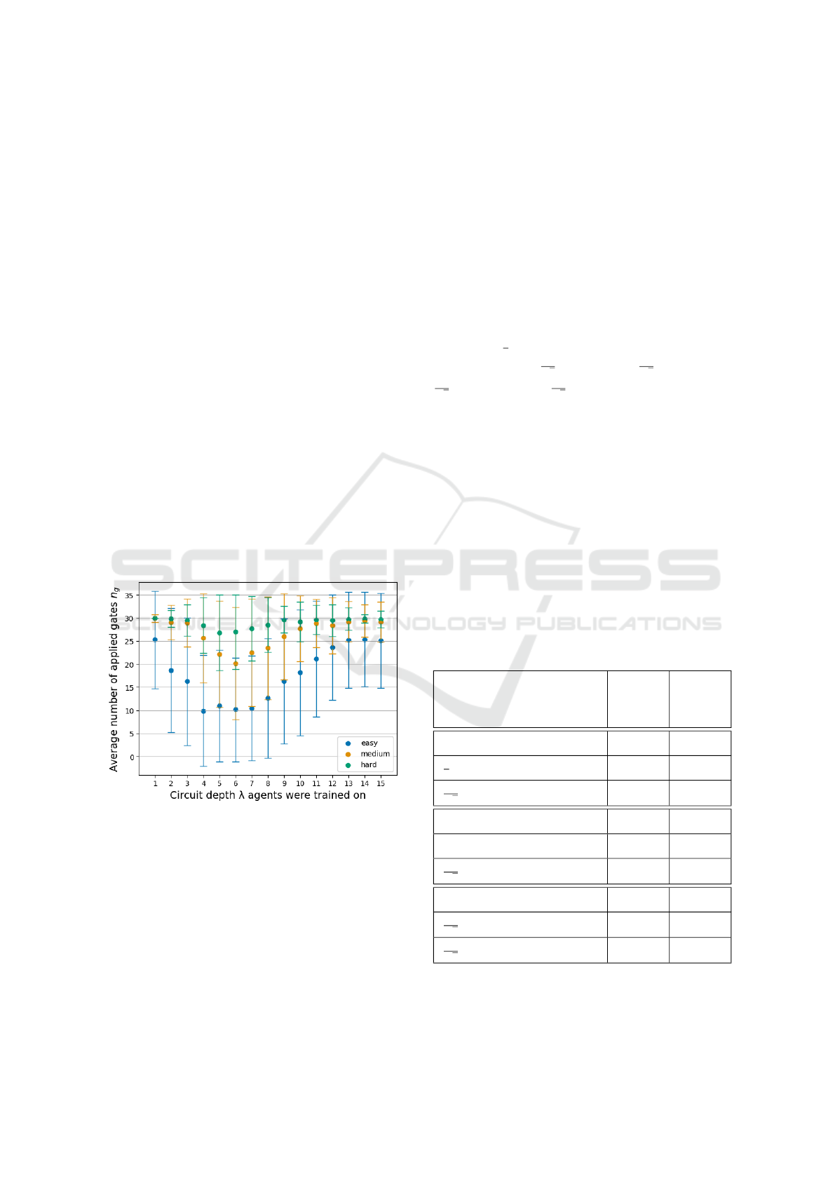
For this experiment, the upper bound of possible ap-
plied actions, corresponding to the maximal calcula-
tion length L was set to 30 steps. It’s evident that each
segment has been successfully solved by at least one
agent with an average gate number below the maxi-
mum step count. When examining the bar chart, sev-
eral trends become apparent. Firstly, there is a clear
correlation between evaluation levels and the average
gate number required for target preparation. Targets
categorized as ’hard’ typically demand more gates, on
average, for their preparation compared to those cate-
gorized as ’medium’ or ’easy.’ This trend arises from
the general need for more gates when dealing with
higher circuit-depth (λ) targets. Another noteworthy
observation pertains to the absence of a shift in peak
performance towards agents trained on high circuit-
depth (λ) targets when transitioning from ’easy’ to
’medium’ and ’hard’ evaluation levels. Intuitively,
one might expect such a shift, given that changing
the evaluation level involves applying agents to target
states with different average circuit-depths (λ). Con-
sequently, it would be reasonable to anticipate a shift
of the best-performing agents towards those trained
on a circuit depth (λ) close to the average circuit-
depth of the respective evaluation level. However, this
expected correlation seems to be lacking, indicating a
weak dependency between these variables.
Figure 5: The average number of gates n
g
applied by PPO-
agents trained on different circuit-depths λ, when applied
on 100 random targets from the evaluation levels ’easy’,
’medium’ and ’hard’ respectively.
The experiment showed a high similarity of the
best-performing agents for the respective evaluation
levels. Specifically, agents trained with λ values
ranging from 4 to 7 exhibited notable performance.
Agents with λ values of 6 and 7 consistently ranked
within the top 3 across all regions, while λ = 5 ap-
peared in the top list of 2 sections. This shared
performance trend may be attributed to the initial
optimization, which emphasized agents with similar
settings. For the subsequent benchmarking of well-
known states, we chose the best-performing agents on
the respective evaluation levels (agents trained with
λ = 4, 5, and 6) as our candidates.
6.2.2 Reconstructing Well-Known States
As mentioned earlier this benchmarking method
again focuses on 2-qubit systems only. We composed
the set out of states well-known in the quantum com-
munity, including the four basis states of the 2-qubit
state-space
|
00
⟩
,
|
01
⟩
,
|
10
⟩
and
|
11
⟩
, the completely
mixed state
1
2
(
|
00
⟩
+
|
01
⟩
+
|
10
⟩
+
|
11
⟩
) and the four
2-qubit bell states
1
√
2
(
|
00
⟩
+
|
11
⟩
),
1
√
2
(
|
00
⟩
−
|
11
⟩
),
1
√
2
(
|
01
⟩
+
|
01
⟩
) and
1
√
2
(
|
01
⟩
−
|
01
⟩
). We divided the
chosen benchmark states into subgroups representing
different levels of evaluation, according to the min-
imal circuit-depth necessary to prepare the respec-
tive states. We obtained the minimal sequences start-
ing from the ground state
|
00
⟩
, using a brute-force
searching algorithm trying all possible combinations
of gates included in the Clifford+T gate set. Accord-
ing to the minimal circuit-depth, we divided the set
into three subgroups (easy: 0-2 gates, medium: 3-4
gates, hard: > 5 gates) The results of this classifi-
cation are displayed in Table 3. Subsequently, we
Table 3: All states included in the 2-qubit set, divided into
subgroups of different evaluation levels, listed together with
the minimal number of quantum gates necessary for their
preparation using only gates contained in the Clifford+T
gate set.
State Minimal
circuit-
depth
Level
|
00
⟩
0 easy
1
2
(
|
00
⟩
+
|
01
⟩
+
|
10
⟩
+
|
11
⟩
) 2 easy
1
√
2
(
|
00
⟩
+
|
11
⟩
) 2 easy
|
01
⟩
4 medium
|
10
⟩
4 medium
1
√
2
(
|
00
⟩
−
|
11
⟩
) 4 medium
|
11
⟩
5 hard
1
√
2
(
|
01
⟩
+
|
10
⟩
) 5 hard
1
√
2
(
|
01
⟩
−
|
10
⟩
) 7 hard
tested agents trained with λ = 4, 5, and 6 on the de-
signed set of states. The outcomes of this investiga-
A Reinforcement Learning Environment for Directed Quantum Circuit Synthesis
91
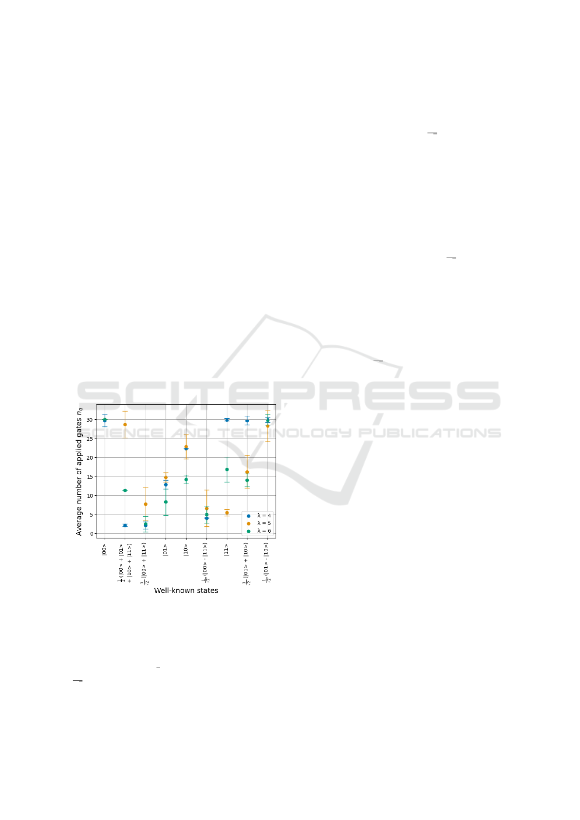
tion are displayed in Fig. 6, while the targets are or-
dered according to the rise in their minimal required
circuit-depth from left to right. An important fact get-
ting evident from the displayed data is the presence of
big performance variations between the agents when
applied to certain targets. Further, the quality of the
agents themselves varies strongly for different tar-
gets. This indicates a form of specialization of certain
agents on specific targets.
For the state
|
00
⟩
, which is equivalent to the initial
state, all tested agents struggle to solve the task. It’s
essential to note that the environment doesn’t check if
the initial state matches the target initially. Hence, in
cases where the target is already reached from the be-
ginning, the agent must apply a gate that preserves the
state, such as S-, T-, or an identity gate on any qubit.
Despite these options comprising more than half of
the available action-space, they are rarely selected, re-
sulting in high n
g
-values. This behavior is explained
by the fact that agents are typically trained on targets
different from the initial state, requiring gates that
modify the current observation. Moreover, due to the
target initialization algorithm’s implementation,
|
00
⟩
is never a target during training when λ ̸= 0. Conse-
quently, agents are explicitly trained to avoid applying
gates that would be useful in this scenario, leading to
suboptimal performance on this specific task.
Figure 6: Performance of PPO-agents trained on circuit-
depths λ = 4,5 and 6 which are applied on the 9 states in-
cluded in the well-known state set given in Table 3.
The λ = 4 agents being trained on a comparatively
low circuit-depth λ show the best results for rela-
tively easy states like
1
2
(
|
00
⟩
+
|
01
⟩
+
|
10
⟩
+
|
11
⟩
) and
1
√
2
(
|
00
⟩
+
|
11
⟩
), while lacking in performance when
applied to the targets of a higher minimal circuit-
depth. On the other hand, agents trained with λ =
5 and 6 are able to perform better on the targets of a
higher minimal circuit-depth, showing strong perfor-
mance in general. For the state
1
√
2
(
|
01
⟩
−
|
10
⟩
) pos-
sessing the highest minimal circuit-depth, all agents
show low potential. To analyze the generated solu-
tions in more detail, the following Table 4 contains
the most promising quantum circuits created within
this benchmark test. We obtained these circuits by
identifying the λ ∈ {4, 5, 6}, which showed the low-
est n
g
for a particular target and subsequently deter-
mined the top-performing agent with the respective
λ. The most frequently generated circuit produced by
this agent was then extracted for the respective tar-
get state. Since the states
|
00
⟩
and
1
√
2
(
|
01
⟩
−
|
10
⟩
)
lead to a wide distribution of created circuits without
a clear favorite, they were excluded from this analy-
sis. The ’Generation probability’ describes the likeli-
hood of occurrence of the specific circuit in percent.
Considering the gates included in the displayed solu-
tions, while bearing in mind the minimal circuit-depth
(see Table 3), it becomes apparent that for all targets
a minimal circuit was found. Further, designs like the
circuit created for
1
√
2
(
|
00
⟩
+
|
11
⟩
) are known to liter-
ature as well (Schneider et al., 2022). The generation
probabilities of the results show that the agents strictly
specialized in the preparation of specific circuits, ob-
taining values of 96-100% for all but one state. Con-
clusively it can be stated that the selected agents per-
form sufficiently on real-world examples as included
in the set, creating highly optimized quantum circuits
which indeed prepare the desired targets.
7 CONCLUSION
In this work, we describe the successful implemen-
tation of a RL environment, enabling the training of
RL agents on the DQCS problem. Relying on the uti-
lization of gates from the Clifford+T gate set only, we
facilitate the direct transfer of the synthesized quan-
tum circuits onto real quantum devices. While ex-
ploring the parameter-space of the DQCS problem,
we demonstrated sufficient task-solving capabilities
of the trained agents, regarding DQCS in a wide vari-
ety of settings. The tested parameter-space spanned
different targets including systems exhibiting qubit
counts of 2, 3, 4, 5, and 10, as well as circuits-depths
ranging from 1 to 15 used for target initialization.
Through the investigation of the agents’ behavior on
different DQCS systems, we discovered correlations
between the target state parameters, qubit-count and
circuit-depth, and the agents reconstructed circuit-
ICAART 2024 - 16th International Conference on Agents and Artificial Intelligence
92
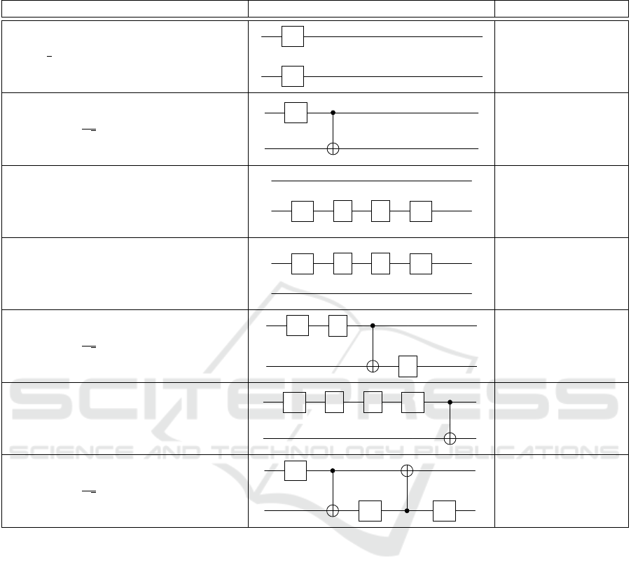
Table 4: States included in the 2-qubit benchmark set listed together with the most probable circuit designs created by the
best-ranked agents.
State Generated circuit Gen. probability [%]
1
2
(
|
00
⟩
+
|
01
⟩
+
|
10
⟩
+
|
11
⟩
)
H
H
100
1
√
2
(
|
00
⟩
+
|
11
⟩
)
H
100
|
01
⟩
H
S S
H
96
|
10
⟩
H
S S
H
98
1
√
2
(
|
00
⟩
−
|
11
⟩
)
H
S
S
76
|
11
⟩
H
S S
H
99
1
√
2
(
|
01
⟩
+
|
10
⟩
)
H
H H
96
depth. It got evident that the reconstructed circuit-
depth increases, if the qubit count or the circuit-depth
is raised. We found 2-qubit targets to be solvable by
the trained agents for a variety of different circuit-
depths. However, the preparation of targets charac-
terized by a qubit number > 2 still poses challenges.
Future efforts could further optimize hyperparam-
eters and refine the agent’s training target-space to
boost RL network performance. We also consider
adopting a curriculum learning or a GAN approach,
with a generative network as the learner and a dis-
criminator for target setting. For quantum computers
using non-Clifford+T gate sets, we’ll integrate param-
eterized gates to devise advanced quantum circuits.
This, however, demands the RL agent to adapt further.
Beyond studying the DQCS issue, we’ve set bench-
marks comparing RL algorithms. Our trained PPO
agents performed on discrete tasks, revealing optimal
circuit designs. We plan to expand these benchmarks
for systems over 2 qubits using k-means clustering.
In summary, our findings demonstrate the appli-
cability and potential of reinforcement learning in ad-
dressing the DQCS problem, highlighting the need
for further research. Our approach represents a sig-
nificant step towards fully automated quantum circuit
synthesis, showcasing the effectiveness of RL meth-
ods in tackling this challenge.
ACKNOWLEDGEMENTS
This work is part of the Munich Quantum Valley,
which is supported by the Bavarian state government
with funds from the Hightech Agenda Bayern Plus.
A Reinforcement Learning Environment for Directed Quantum Circuit Synthesis
93

REFERENCES
Altmann, P., B
¨
arligea, A., Stein, J., K
¨
olle, M., Gabor, T.,
Phan, T., and Linnhoff-Popien, C. (2023). Challenges
for reinforcement learning in quantum computing.
Barenco, A., Bennett, C. H., Cleve, R., DiVincenzo,
D. P., Margolus, N., Shor, P., Sleator, T., Smolin,
J., and Weinfurter, H. (1995). Elementary gates for
quantum computation. Phys.Rev. A52 (1995) 3457,
52(5):3457–3467.
Bennett, C. H. and Wiesner, S. J. (1992). Communica-
tion via one- and two-particle operators on einstein-
podolsky-rosen states. Phys. Rev. Lett., 69:2881–
2884.
Blazina, D., Duckett, S. B., Halstead, T. K., Kozak, C. M.,
Taylor, R. J. K., Anwar, M. S., Jones, J. A., and
Carteret, H. A. (2005). Generation and interrogation
of a pure nuclear spin state by parahydrogen-enhanced
nmr spectroscopy: a defined initial state for quantum
computation. Magn. Reson. Chem., 43(3):200–208.
Cerezo, M., Arrasmith, A., Babbush, R., Benjamin, S.,
Endo, S., Fujii, K., McClean, J., Mitarai, K., Yuan,
X., Cincio, L., and Coles, P. J. (2021). Variational
quantum algorithms. Nat Rev Phys, 3:625–644.
Ekert, A. K. (1991). Quantum cryptography based on bell’s
theorem. Phys. Rev. Lett., 67(6).
Farhi, E. and Neven, H. (2018). Classification with quan-
tum neural networks on near term processors. arXiv:
Quantum Physics.
F
¨
osel, T., Niu, M. Y., Marquardt, F., and Li, L. (2021).
Quantum circuit optimization with deep reinforce-
ment learning.
Gabor, T., Zorn, M., and C., L.-P. (2022). The applicabil-
ity of reinforcement learning for the automatic gener-
ation of state preparation circuits. GECCO ’22: Pro-
ceedings of the Genetic and Evolutionary Computa-
tion Conference Companion, page 2196–2204.
Jozsa, R. (1994). Fidelity for mixed quantum states. Journal
of Modern Optics, 41(12):2315–2323.
Kaye, P., Laflamme, R., and M., M. (2007). An Introduction
to Quantum Computing. Oxford University Press.
Krenn, M., Kottmann, J. S., Tischler, N., and Aspuru-
Guzik, A. (2021). Conceptual understanding through
efficient automated design of quantum optical experi-
ments. Phys. Rev. X, 11.
Krenn, M., Malik, M., Fickler, R., Lapkiewicz, R., and
Zeilinger, A. (2015). Automated search for new quan-
tum experiments. Phys. Rev. Lett. 116, 090405 (2016),
116(9):090405.
Li, Z., Peng, J., Mei, Y., Lin, S., Wu, Y., Padon, O., and Jia,
Z. (2023). Quarl: A learning-based quantum circuit
optimizer.
Mackeprang, J., Dasari, D. B. R., and Wrachtrup, J.
(2019). A reinforcement learning approach for quan-
tum state engineering. Quantum Machine Intelligence
2, 1(2020), 2(1).
Mansky, M. B., Castillo, S. L., Puigvert, V. R., and
Linnhoff-Popien, C. (2022). Near-optimal circuit con-
struction via cartan decomposition.
Mnih, V., Badia, A. P., Mirza, M., Graves, A., Lillicrap,
T. P., Harley, T., Silver, D., and Kavukcuoglu, K.
(2016). Asynchronous methods for deep reinforce-
ment learning. ICML 2016.
Nielsen, M. A. and Chuang, I. L. (2010). Quantum com-
putation and quantum information. 10th anniversary
edition. Cambridge: Cambridge University Press.
Ostaszewski, M., Trenkwalder, L. M., Masarczyk, W.,
Scerri, E., and Dunjko, V. (2021). Reinforcement
learning for optimization of variational quantum cir-
cuit architectures. Advances in Neural Information
Processing Systems (NeurIPS 2021), 34.
Parlett, B. (2000). The qr algorithm. Computing in Science
& Engineering, 2(1):38–42.
Peruzzo, A., McClean, J., Shadbolt, P., Yung, M.-H., Zhou,
X.-Q., Love, P. J., Aspuru-Guzik, A., and O’Brien,
J. L. (2013). A variational eigenvalue solver on a
quantum processor. Nature Communications, 5:4213,
(2014), 5(1).
Pirhooshyaran, M. and Terlaky, T. (2021). Quantum circuit
design search. Quantum Machine Intelligence, 3(25).
Puterman, M. L. (2014). Markov decision processes: dis-
crete stochastic dynamic programming. John Wiley &
Sons.
Schneider, S., Burgholzer, L., and Wille, R. (2022). A sat
encoding for optimal clifford circuit synthesis. ASP-
DAC ’23: Proceedings of the 28th Asia and South Pa-
cific Design Automation Conference, page 190–195.
Schuld, M., Bocharov, A., Svore, K., and Wiebe, N. (2020).
Circuit-centric quantum classifiers. Phys. Rev. A, 101.
Schulman, J., Wolski, F., Dhariwal, P., Radford, A., and
Klimov, O. (2017). Proximal policy optimization
algorithms. International Conference on Machine
Learning (ICML).
T
´
oth, G. and Apellaniz, I. (2014). Quantum metrology from
a quantum information science perspective. J. Phys.
A: Math. Theor., 47(42).
Xu, M., Li, Z., Padon, O., Lin, S., Pointing, J., Hirth, A.,
Ma, H., Palsberg, J., Aiken, A., Acar, U. A., and
Jia, Z. (2022). Quartz: Superoptimization of quan-
tum circuits. Association for Computing Machinery,
43:625–640.
Zhang, X.-M., Wei, Z., Asad, R., Yang, X.-C., and Wang,
X. (2019). When does reinforcement learning stand
out in quantum control? a comparative study on state
preparation. npj Quantum Inf, 5(85).
ICAART 2024 - 16th International Conference on Agents and Artificial Intelligence
94
