Nearest Neighbor-Based Data Denoising for Deep Metric Learning
George Galanakis
1,2 a
, Xenophon Zabulis
2 b
and Antonis A. Argyros
1,2 c
1
Computer Science Department, University of Crete, Greece
2
Institute of Computer Science, FORTH, Greece
Keywords:
Label Noise, Data Denoising, Deep Metric Learning, KNN, Image Retrieval.
Abstract:
The effectiveness of supervised deep metric learning relies on the availability of a correctly annotated dataset,
i.e., a dataset where images are associated with correct class labels. The presence of incorrect labels in a
dataset disorients the learning process. In this paper, we propose an approach to combat the presence of such
label noise in datasets. Our approach operates online, during training and on the batch level. It examines the
neighborhood of samples, considers which of them are noisy and eliminates them from the current training
step. The neighborhood is established using features obtained from the entire dataset during previous training
epochs and therefore is updated as the model learns better data representations. We evaluate our approach using
multiple datasets and loss functions, and demonstrate that it performs better or comparably to the competition.
At the same time, in contrast to the competition, it does not require knowledge of the noise contamination rate
of the employed datasets.
1 INTRODUCTION
Two of the most common tasks related to analysis of
images are classification and retrieval. In their sim-
pler form, they both operate on the image level. In
classification the task is to associate the image with a
class/label from a predefined set of classes, while in
retrieval the goal is to identify a set of similar images
from an existing database, in ranked order. In many
practical scenarios, classes are not known beforehand;
In other situations, lack of existing data may result to
inaccuracies. Therefore, a classifier learned on a pre-
defined set of classes is not possible. Instead of learn-
ing a classifier, retrieval approaches, usually posed as
metric learning, operate on the relative similarity of
images and aim to construct embedding spaces where
similar ones lay in nearby areas, while dissimilar im-
ages are far apart. In this work we focus on the re-
trieval and, more specifically, in the case in which
there is noise noise in the training dataset.
Despite the emergence of off-the-self pre-trained
models and the availability of self-supervised and
few-shot learning approaches, the majority of ma-
chine learning algorithms are still data-hungry and re-
quire excessive annotation efforts. Annotation can be
a
https://orcid.org/0000-0002-6261-6252
b
https://orcid.org/0000-0002-1520-4327
c
https://orcid.org/0000-0001-8230-3192
performed either by humans or by some (semi-) auto-
matic approaches. In both cases, annotated data might
contain errors. Causes of these errors are misunder-
standing, ambiguity or other human and machine in-
herent issues that arise during the annotation process.
In the context of this work we are interested in
annotation errors with respect to labels that are as-
sociated with images. For example, an image might
be assigned a label that does not correspond to the
correct object class, e.g. an image is associated with
a dog class but it actually depicts a cat. Our pro-
posed methodology, called Nearest Neighbor-based
Data Denoising (N2D2) deals with such or similar
types of noise in an online fashion. It identifies the
noisy samples that are contained in the current train-
ing batch and eliminates them from the computation
of the loss, such that they do not negatively affect the
training of the model.
The basic idea behind our approach is depicted in
Fig. 1. The left part of the figure illustrates a clean
dataset comprised of 3 classes, “a”, “b” and “c”, while
the right part the same dataset where 2 samples, (1)
and (3), are mislabeled. Suppose that we want to ex-
amine samples (1)-(3) that are contained in the current
training batch. The samples are assigned with scores
and are classified as noisy or clean - see the method-
ology section for details. In this case, (1) is correctly
identified as noisy; a fairly simple task. Sample (2)
Galanakis, G., Zabulis, X. and Argyros, A.
Nearest Neighbor-Based Data Denoising for Deep Metric Learning.
DOI: 10.5220/0012383000003660
Paper published under CC license (CC BY-NC-ND 4.0)
In Proceedings of the 19th International Joint Conference on Computer Vision, Imaging and Computer Graphics Theory and Applications (VISIGRAPP 2024) - Volume 2: VISAPP, pages
595-603
ISBN: 978-989-758-679-8; ISSN: 2184-4321
Proceedings Copyright © 2024 by SCITEPRESS – Science and Technology Publications, Lda.
595

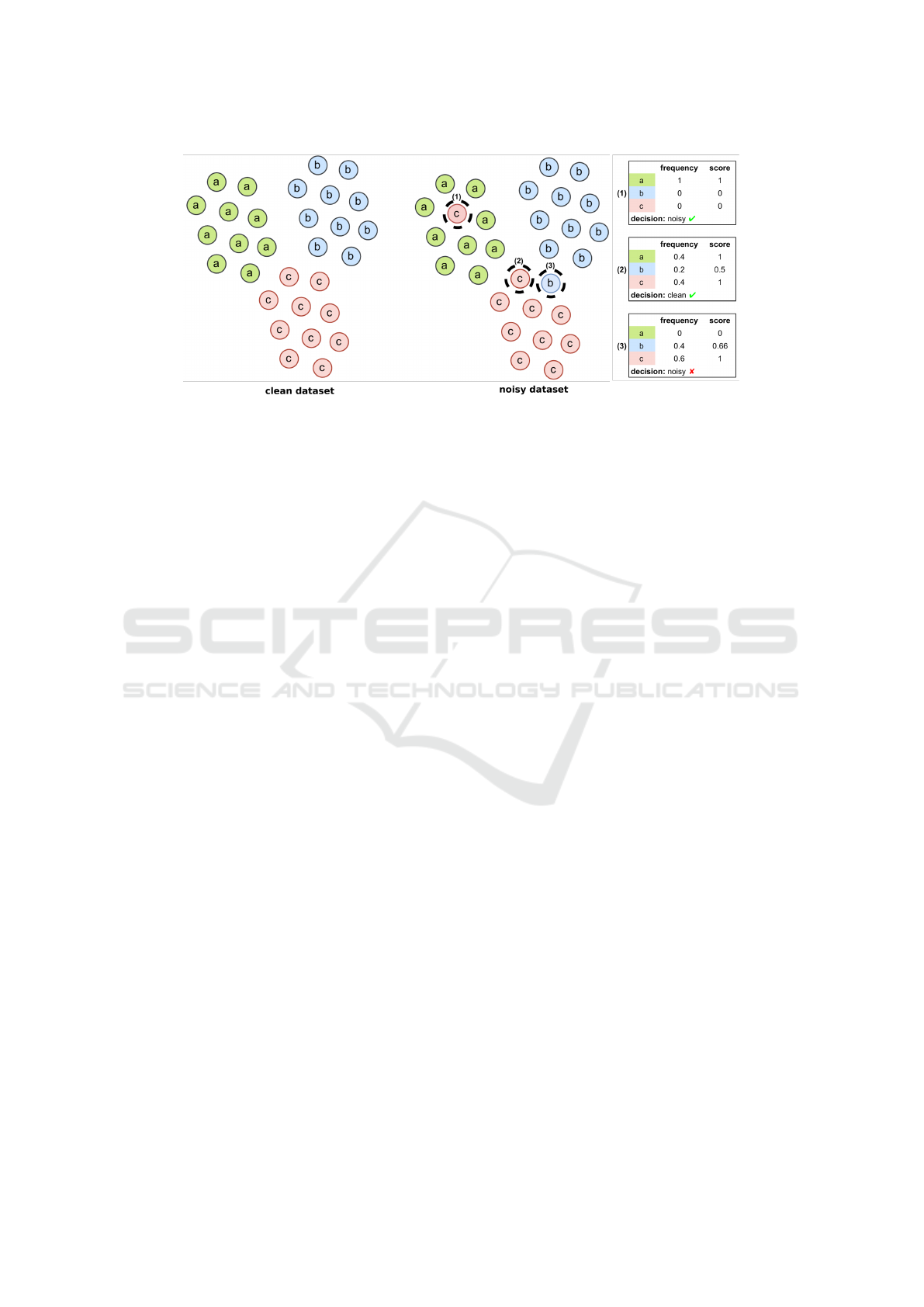
Figure 1: A simple example of the identification of samples as noisy versus clean using our method. See text for details.
is correctly identified as clean despite the presence of
the other samples among the neighbors. (3) is a corner
case, where a noisy sample is identified as clean.
2 RELATED WORK
Noise Types. The existence of falsely labeled train-
ing samples is usually referred to as label noise. A
common labeling mistake, especially existent in large
datasets, is the assignment of an image to a wrong
class. Other types of disturbances in the appearance
of the object can also be considered as noise. Such
disturbances include occlusions of the dominant ob-
ject, co-existence of multiple objects corresponding
to either known or unknown classes, random sensor
noise, etc. The above types of noise have been also
reported as label noise, in the sense that the single la-
bel that is assigned does not represent the entire story
told by the image.
The above types of noise can be found in both syn-
thetic and real-world noisy datasets that have been ex-
ploited by recent noise-aware methodologies. A syn-
thetic dataset can be created by random mutation of
some of the correct labels of an existing clean dataset,
with the mutation being either symmetric - same num-
ber of images from all classes mutate to noisy - or
asymmetric. Another type of synthetic noise, called
small-cluster noise, was introduced by (Liu et al.,
2021). This type of noise eliminates some of the
known classes by randomly assigning corresponding
images to the rest of the classes. This process im-
itates an openset scenario, where images from un-
known classes are present in the data. On the other
hand, real-world datasets are usually crawled without
supervision from random internet sources, and there-
fore noise is inherent.
Noise in Classification Problems. Combating la-
bel noise during training of neural networks has been
studied mostly for classification problems. A popular
family of such methods is called Co-teaching (Han
et al., 2018), which suggested the paradigm of simul-
taneously training two identical networks. The main
idea is to update the one model based on observations
of the other model. More specifically, the set of batch
samples that have small loss when passed through
the one network are used to update the weights of
the companion network. This approach aims to find
noisy samples by reducing the bias that each indi-
vidual network has on the samples that it has pre-
viously seen. An extension of this approach, called
Co-teaching+ (Yu et al., 2019), first considers sam-
ples from which the two classifiers disagree on the
predicted label and then selects the subset of samples
that have small loss. Disagreement helps the two net-
works stay divergent during training, else they con-
verge to the same solution and essentially degener-
ate to the same network. The approach in (Xia et al.,
2020) proposed a method to distinguish the critical
parameters and non-critical parameters of the network
and applied different update rules for different types
of parameters. This is based on the observation that
non-critical ones tend to overfit noisy labels and their
gradients are misleading for generalization. The work
in (Yao et al., 2021) proposed the Jensen-Shannon di-
vergence as measure between the correct labels dis-
tribution and the predicted one in order to identify
the noisy samples. They also have a separate pro-
cess for distinguishing in-distribution (ID) and out-
of-distribution (OOD) noise samles and they re-label
the ID samples according to a proposed label that is
obtained from a mean-teacher network.
A more recent method called SSR (Feng et al.,
2022) combines classification prediction and inspec-
tion of the feature space neighborhood of the samples.
VISAPP 2024 - 19th International Conference on Computer Vision Theory and Applications
596

First, samples whose classification score is above a
threshold but their label is not the same, are relabeled
accordingly. Afterwards, a sample is considered as
clean if the most popular label among its neighbors
is the same as that of the sample. Both sample rela-
beling and noise removal processes are applied to the
entire dataset, after each training epoch. Our method
is similar to SSR in the sense of the use of K Near-
est Neighbor (KNN) for determining noisy samples.
However, we apply our method in the context of re-
trieval, we do not apply any re-labeling mechanism
and also we utilize an alternative scoring methodol-
ogy for determining noisy samples.
Noise in Metric Learning Problems. Deep met-
ric learning approaches are closely related to the
loss function that is used for learning the embedding
space. Some of the loss functions are purposefully
designed do deal with label noise. For example, Sub-
Center ArcFace (Deng et al., 2019) loss extends the
ArcFace loss (Deng et al., 2019) with multiple cen-
ters per-class, such that presence of noisy samples
does not affect considerably the single learned cen-
troid. SoftTriple loss (Qian et al., 2019) shares the
same idea for multiple centers and is inherently more
robust against label noise, however it was not origi-
nally evaluated on noisy datasets. Most recently, CCL
(Cai et al., 2023) adopts the same idea about maintain-
ing a center bank. However, it utilizes a contrastive
loss. We evaluate our method using both robust and
non-robust losses and report the impact in each case.
Since CCL was only recently proposed and its imple-
mentation was not available, we did not include it in
our experiments.
Explicit consideration and elimination of noisy
samples is a less studied topic. Two recent approaches
are PRISM (Liu et al., 2021) and T-SINT (Ibrahimi
et al., 2022). PRISM maintains a memory queue
of the features of all samples and one centroid per
class. Samples are compared using the cosine sim-
ilarity metric against their corresponding class cen-
troid and those with low similarity that fall under a
filtering ratio are considered as noisy. The memory
queue is filled up with samples that are considered
clean. T-SINT proposed a student-teacher architec-
ture, where the teacher model identifies noisy sam-
ples in the pairwise distance matrix and appropriately
guides the student network to update its weights. T-
SINT operates directly on the distance matrix and ex-
cludes only the false positive pairs, i.e. positive pairs
that include the noisy samples. A common shortcom-
ing of PRISM and T-SINT is that they require knowl-
edge of the noise rate of the dataset, which is a strong
requirement.
In practice, T-SINT operates very similarly to
PRISM in the datasets which we consider for bench-
marking, while its performance gain is attributed to
the better network architecture it utilizes. Further-
more, it can be considered as a more intrusive method
with respect to the current implementations as it de-
pends on two concurrent networks (student-teacher)
and the source code for fair comparison is not pro-
vided. Hence, we chose PRISM as a baseline com-
petitor.
Our method shares some similarities and differ-
ences with PRISM. Both methods keep a memory
bank of the features during training. PRISM does so
for updating the class centroids during training. In-
stead, we use the entire bank once, at the end of each
epoch, to establish the similarities between all dataset
samples as required for the inspection of batch sam-
ples’ neighborhood in subsequent steps. Also, both
methods are not directly dependent to the neural net-
work and loss, thus can be applied as an extension to
already robust networks and losses. A core difference
of our method is that it does not require the knowl-
edge of the filtering rate to determine noisy samples
as PRISM does.
The contributions of the present work can be sum-
marized as follows.
• This work presents a method about accounting
label noise during supervised training of deep
metric learning models through exploration of
the neighborhood of the batch samples using the
KNN algorithm.
• Our method is evaluated against baselines and
the competing PRISM approach on a range of
datasets, noise rates and types. It is demonstrated
that in most cases, it performs better than PRISM
even with less information than their method re-
quires, i.e. the noise rate of the dataset.
• The method is decoupled with respect to the neu-
ral network architecture and the loss function,
thus, in contrast to other proposed methodolo-
gies, it can be plugged into any existing training
pipeline as a preceding step before the computa-
tion of the loss and/or mining processes.
3 METHODOLOGY
The general training pipeline of deep metric models
includes the following steps (forward pass): (a) pop-
ulation of samples of a batch through a sampling
method, (b) feeding the samples through the net-
work and extraction of features, (c) mining of pairs or
triplets and, (d) computation of the loss. Let X denote
the features of the batch samples of size N ×D, where
Nearest Neighbor-Based Data Denoising for Deep Metric Learning
597

input : training batch B containing features
X of size N × D and labels y of size
N; noise predictor P
n
output: noise prediction pred of size N
1 assign pred with all f alse
2 if P
n
has not trained then
3 return pred;
4 else
5 foreach x
i
, y
i
in B do
6 /* P
n
pipeline */
7 Find k neighbors of x
i
;
8 Calculate scores s;
9 if s(y
i
) < θ then
10 pred(i) ←− true
11 end
12 return pred;
Algorithm 1: Overview of the proposed algorithm for the
identification of noisy samples.
N is the batch size and D the dimensionality of the
features. Let also y denote the corresponding labels
of a total number of C classes that are contained in the
dataset. We propose extending this pipeline by intro-
ducing an extra step, after features extraction, which
considers if the samples are noisy or not and reduces,
quite similar to mining, the samples that will be con-
sidered for computing the loss. We denote such noise
predictor module as P
n
.
3.1 Identification of Noisy Samples
Our methodology for identifying noisy samples relies
on the realization that the neighborhood of a sample
in the embedding space should mostly contain sam-
ples which correspond to the same class. From an-
other perspective, noisy samples i.e., samples that are
mislabelled, are expected to be surrounded by neigh-
bors that mostly correspond to other classes. How-
ever, the above assumption holds only when the em-
bedding space has been considerably formed, mean-
ing that samples from the same class are close to each
other, while samples from different classes lay further
apart.
In order to quantify the purity of the neighborhood
of a sample, we obtain statistics of the nearest neigh-
bors. More specifically, we count the k nearest neigh-
bors and normalize over k. We then construct a C
dimensional vector, containing the frequency of each
class into the neighborhood of the sample, as obtained
previously. Finally we scale the vector into the range
[0, 1], to compensate for various neighborhood con-
figurations. Classification of a sample as noisy is then
as simple as comparing the score of its correspond-
ing class against a threshold θ; we choose θ = 0.5. If
the score of the sample is lower than the threshold, it
means that the neighborhood does not support the la-
bel of the class and therefore we consider it as noisy.
The above steps are summarized in Algorithm 1.
At every training iteration, X, y are kept in a mem-
ory bank. In the end of all iterations (epoch end) we
index the training data using FAISS library (Johnson
et al., 2019), which permits fast computation of the k
nearest neighbors in subsequent steps.
3.2 Loss Functions
A key aspect in metric learning is the loss function
which guides the evolution of the embedding space
through training. The loss function endorses small
distances between same-class samples and large dis-
tances between samples that correspond to different
classes. As it has been demonstrated, some losses are
more resistant than others when they encounter label
noise, while others work better on different types of
noise. In this work we explore different losses in or-
der to demonstrate the effectiveness of our approach
in such different scenarios. We briefly describe the
losses below.
Contrastive Loss. The baseline of metric learning
losses is the Contrastive Loss, given by Eq.1.
L
contrastive
= [d
p
− m
pos
]
+
+ [m
neg
− d
n
]
+
(1)
The loss penalizes large intra-class distances (d
p
) and
small inter-class distances (d
n
), of the samples that
appear in the training batch, given margins that regu-
late the amount of the penalty that is applied; by de-
fault m
pos
= 0.0 and m
neg
= 1.0.
Cross-Batch Memory Loss. Cross-Batch Memory
Loss (XBM) (Wang et al., 2020) was proposed as an
extension to Contrastive Loss, as it aims to increase
the number of pairwise distances, by not only com-
paring samples within batch but also across batches.
This approach essentially provides more appropriate
negative examples which are crucial for learning. For
this purpose, it keeps a memory bank containing em-
beddings and corresponding labels from the previous
batches. The memory bank is implemented as a FIFO
queue, containing n most recent embeddings, where n
is a hyperparameter.
Multi-Similarity Loss. Multi-Similarity Loss (Wang
et al., 2019) is formulated as
L
MS
=
1
m
m
∑
i=1
{
1
a
log[1 +
∑
k∈P
i
e
−a(S
ik
−λ)
]
+
1
β
log[1 +
∑
k∈N
i
e
β(S
ik
−λ)
]},
(2)
VISAPP 2024 - 19th International Conference on Computer Vision Theory and Applications
598

Table 1: Statistics of the datasets.
Dataset
Training set
# classes / samples
Testing set
# classes / samples
MNIST / KMNIST 10 / 60,000 10 / 10,000
Cars 98 / 8,054 98 / 8,131
CUB 100 / 5,864 100 / 5,924
SOP 11,318 / 59,551 11,316 / 60,502
where a,β, λ are hyperparameters. For each anchor-
negative pair, this loss considers both the similarity
of the samples in this pair (self-similarity), but also a
relative similarity with respect to other negative pairs.
The same holds for positive pairs, too. In such way,
the impact of each pair in the loss is weighted accord-
ing to both self and relative similarities with respect
to other pairs of samples.
SoftTriple Loss. SoftTriple Loss (Qian et al., 2019),
is a proxy-based loss inspired by the Softmax loss,
which is common in classification, and the triplet loss.
It maintains multiple learnable centers for each class
(proxies) and replaces the standard sample-sample
similarity with a weighted sample-proxies similarity.
Essentially, the proxies can be thought of as learnable
representatives of each class.
L
ST
(x
i
) = − log
exp(λ(S
′
i,y
i
− δ))
exp(λ(S
′
i,y
i
− δ)) +
∑
j̸=y
i
exp(λS
′
i, j
)
,
(3)
where
S
′
i,c
=
∑
k
exp(
1
γ
x
T
i
w
k
c
)
∑
k
exp(
1
γ
x
T
i
w
k
c
)
x
T
i
w
k
c
. (4)
In the above equation, x
i
is the i-th batch sample and
w
k
c
represents the k-th proxy of class c. γ, δ are prede-
fined hyperparameters.
Sub-center ArcFace Loss. Sub-center ArcFace Loss
(SCAF) (Deng et al., ) is an extension to the popular
ArcFace Loss (Deng et al., 2019) and shares a simi-
lar idea to SoftTriple by utilizing multiple centers per
class, hence the name “Sub-center”.
L
SCAF
= − log
e
scos(θ
i,y
i
+m)
e
scos(θ
i,y
i
+m)
+
∑
N
j=1, j̸=y
i
e
scos θ
i, j
, (5)
where
θ
i, j
= arcos(max
k
(W
T
jk
x
i
)), k ∈ {1, . . . , K}. (6)
In the above equation, K represents the number of
centers per class and θ
i j
the angle of feature vectors
that represent i-th and j-th samples. m and s are hy-
perparameters. As stated in (Deng et al., ), the loss
can compensate possible noise in datasets due to the
multiple centers per-class.
Some of the loss functions above might bene-
fit from reasoning about which positive and negative
samples should be accounted, for computing the loss
of a given batch sample. This operation is commonly
referred as online pair/triplet mining. We did not
adopt any mining algorithm for two reasons. First,
to retain a common basis of comparison and second,
to reduce the overhead of comparing with and with-
out an additional algorithmic parameter. We note that
our scope is not towards exhaustive evaluation of met-
ric losses, but to demonstrate that our method benefits
few recent of them.
4 EXPERIMENTS
4.1 Datasets
We evaluate our method on four datasets, MNIST
(LeCun and Cortes, 2010), Stanford Cars (Krause
et al., 2013), Caltech-UCSD Birds-200-2011 (CUB)
(Wah et al., 2011) and Stanford Online Products
(SOP) (Oh Song et al., 2016). Cars and CUB datasets
were originally created for the classification task,
meaning that training and testing set share the same
classes. We use the re-organized splits provided
by (Liu et al., 2021). For MNIST, rather than re-
organizing the dataset we used an alternative one
called Kuzushiji-MNIST (KMNIST) (Clanuwat et al.,
2018) to serve as the testing set. KMNIST comprises
of 10 characters of Japanese cursive writing style and
was proposed as a drop-in replacement of MNIST.
Tab.1 shows the dataset statistics and Fig.2 demon-
strates indicative images of them. Each dataset is
evaluated for varying synthetic noise rates.
4.2 Implementation & Training Settings
We implemented our method using PyTorch Light-
ning framework (Falcon, 2019). We also adopted im-
plementations of loss functions from PyTorch Metric
Learning library (Musgrave et al., 2020b). Comple-
mentary to our algorithm, we re-implemented PRISM
(Liu et al., 2021), in order to have a common ex-
perimental framework and maintain the same settings
across multiple runs. We validated the implementa-
tion using Cars dataset and 50% noise rate.
As it is stated in (Musgrave et al., 2020a), the
curse of metric learning approaches is that they are
not compared under the same settings and, most im-
portantly, that performance improvements are actu-
ally due to different training settings and modeling
rather than the proposed methodologies themselves.
With this in mind, our experimentation was conducted
in a way to guarantee accurate comparison of the
Nearest Neighbor-Based Data Denoising for Deep Metric Learning
599

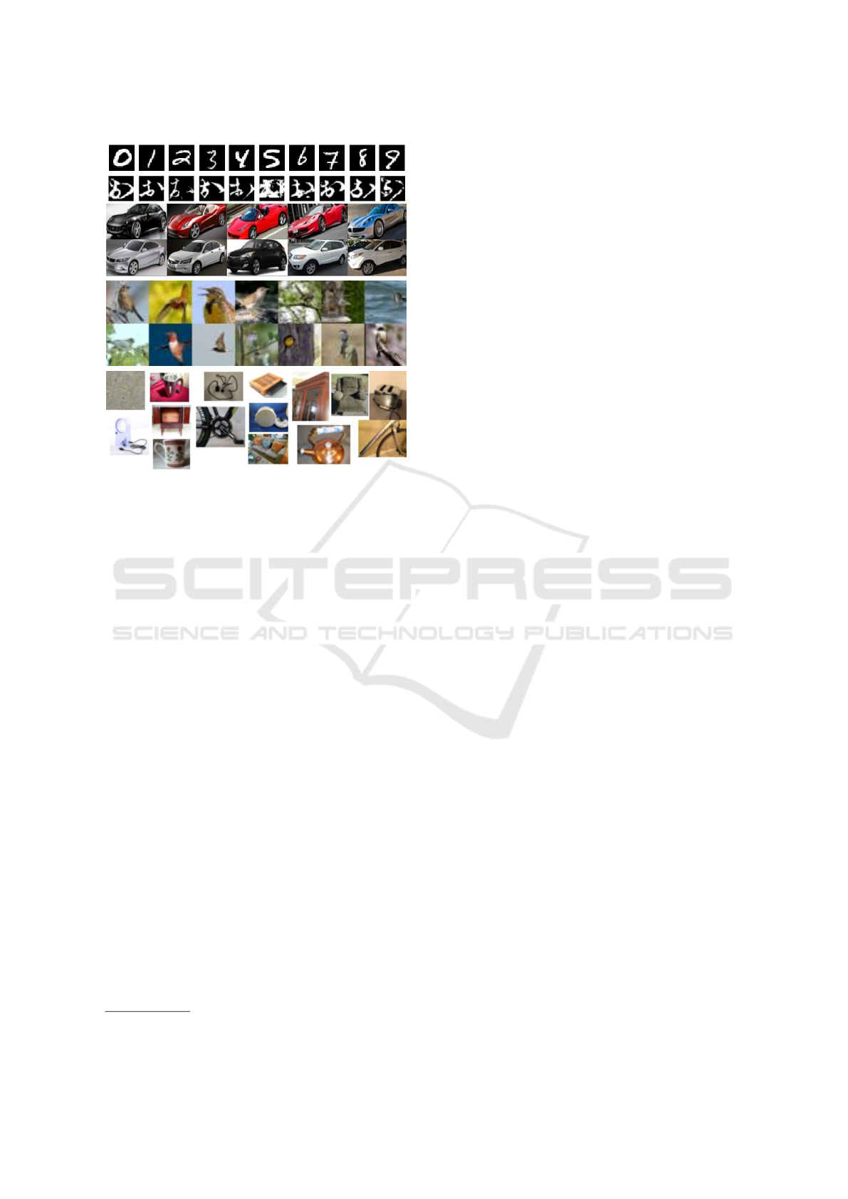
Figure 2: Indicative samples from the evaluated datasets.
From top to bottom: MNIST & KMNIST, Cars, CUB and
SOP.
noise reduction methodologies and we did not opti-
mize or fine-tuned the settings for each dataset. We
fixed the random seed for all experiments, too.
For the experiments which include Cars, CUB and
SOP datasets, our training settings mirror those spec-
ified in (Liu et al., 2021). More specifically, for Cars
and CUB we utilize the BN-Inception CNN architec-
ture for learning 512-d embeddings while for SOP we
utilize ResNet-50 with an additional 128-d linear pro-
jection head. Each model is trained for 30 epochs us-
ing Adam optimizer with initial learning rate 3
−5
and
weight decay 5
−4
. For the losses which include train-
able parameters, namely SoftTriple and Sub-center
ArcFace, we utilized the same optimizer as the base
model however with higher learning rate as suggested
in (Qian et al., 2019). At each training step the learn-
ing rate is updated using the Cosine Annealing ap-
proach (Loshchilov and Hutter, 2016). During train-
ing, each sample is randomly resized and flipped on
the horizontal axis. The batch size is set to 64, while
each batch is formed using at least 4 samples of the
same class, such that there are enough positive exam-
ples to be used by the loss.
For the experiments on MNIST, we utilize a much
simpler model comprising of 2 linear layers, where
each layer is followed by ReLU and Dropout opera-
tions. The embeddings are 64-d and are obtained from
the top layer. All implementation details can be found
in the provided code
1
.
1
github.com/ggalan87/nearest-neighbor-data-denoising
4.3 Evaluation Criteria
For evaluating our method, we follow the standard
protocol that is applied in the domain of metric learn-
ing. We utilize a testing set which is disjoint to
the training set with respect to class labels; i.e., no
class of training set appears in the test set. More
specifically, we adopted the dataset splits that were
provided by (Liu et al., 2021). After training, em-
beddings of the testing set are extracted and nearest
neighbors of each sample are computed and ranked.
Given the ranked list, we compute and report Preci-
sion@1 (P@1), as the evaluation metric. Following
(Liu et al., 2021), we report the result of the best per-
forming model.
4.4 Results & Discussion
Results of the experimental evaluation using various
loss functions and noise rates are demonstrated in Ta-
bles 2-3. Both our approach and PRISM, being au-
tonomous noise reduction models, directly operate on
the current batch of training samples and decide if a
sample is noisy or not based on historical observations
and statistics. In order to have an upper limit of the
effect of such approach we also run the same exper-
iments using a ground-truth noise reduction model.
This model is given the correct noisy samples and
therefore constructs a ground-truth filter.
We note that a core hyperparameter of PRISM al-
gorithm is the filtering rate, which is the amount of
samples that will be considered for removal. We in-
sist that this is a hard requirement. Since PRISM does
not explicitly specify the noise rates for which their
experiments were run, we include results from runs
of PRISM with (a) filtering rate fixed to the ground-
truth noise rate of the dataset but also (b) runs where
the filtering rate is set to an arbitrary value i.e., 50%.
Small and Medium Scale Datasets. Table 2 shows
the results of the experiments that were run on
MNIST, Cars and CUB datasets. In the majority
of the experiments, our method obtained better P@1
than PRISM, while in the rest of the experiments,
it operated on par. We note that our method has a
great advantage in that it does not require the knowl-
edge of the noise rate as PRISM does. More specif-
ically, in the experiments with the Cars dataset, our
method obtained the highest P@1 for all noise rates
and noise types. In MNIST and CUB our method re-
sulted in equivalent P@1 and at least a combination
of our method and a loss function is the second best
and very close to the best approach.
VISAPP 2024 - 19th International Conference on Computer Vision Theory and Applications
600

Table 2: Label noise experiments on CARS, CUB, and MNIST datasets. In the case of PRISM, dual results correspond to a
correct and a 50% noise rate (hyperparameter of method). See text for the details. The reported result is Precision@1. The
best score excluding ground-truth noise removal is annotated with bold font, while the second best with underline.
MNIST −→ KMNIST CARS CUB
symmetric noise symmetric noise small cluster noise symmetric noise small cluster noise
loss name 10% 20% 50% 10% 20% 50% 25% 50% 10% 20% 50% 25% 50%
without noise reduction
XBM 95.41 94.63 91.8 76.95 74.36 67.23 72.17 62.8 54.25 54.34 49.61 52.45 48.75
MS 96.42 95.77 94.13 76.29 69.98 43.02 69.72 46.03 56.03 53.48 33.46 51.23 37.73
SCAF 95.98 95.42 92.98 78.2 67.07 54.71 65.36 64.28 56.11 54.19 45.93 54.51 45.8
ST 96.23 95.86 94.35 76.22 72.85 61.14 74.74 68.43 54.32 52.87 46.3 53.44 49.73
ground-truth noise reduction
XBM 94.84 94.79 94.12 77.61 77.35 75.01 76.97 70.73 54.68 54.95 53.98 54.61 55.72
MS 96.22 96.28 96.02 78.35 78.39 73.81 76.72 72.46 55.72 55.44 54.27 51.16 50.03
SCAF 96.38 96.53 95.71 81.29 80.56 76.88 77.91 74.06 56.95 57.33 54.2 53.97 55.01
ST 97.16 97.06 96.63 80.3 79.26 74.08 78.7 75.07 57.26 56.55 53.83 51.23 52.84
PRISM (50% noise rate)
XBM 92.21 92.22 92.2 71.21 72.47 73.44 70.99 65.99 53.06 53.39 51.96 52.41 50.57
MS 91.88 89.63 86.81 67.99 69.98 69.57 68.9 68.55 50.56 52.18 52.79 51.52 49.65
SCAF 91.99 91.71 94.22 73.78 75.06 53.29 72.15 70.64 54.12 53.81 53.29 53.17 49.54
ST 93.34 92.98 93.91 75.29 75.65 69.14 75.48 71.7 55.62 55.86 51 53.81 51.4
PRISM (correct noise rate)
XBM 94.44 94.16 92.2 77.57 76.58 73.44 75.19 65.99 54.71 55.64 51.96 53.87 50.57
MS 95.71 94.06 86.81 78.49 76.5 69.57 75.03 68.55 55.98 55.55 52.79 53.71 49.65
SCAF 96.14 95.9 94.22 79.84 78.86 53.29 77.64 70.64 56.95 57.14 53.29 54.71 49.54
ST 96.58 96.27 93.91 79.13 77.07 69.14 76.9 71.7 56.4 54.95 51 54.66 51.4
N2D2 (ours)
XBM 94.22 93.82 91.8 76.05 74.1 71.8 73.83 64.8 55.3 55.5 54.19 54.61 51.35
MS 94.17 93.58 92.56 74.08 74.8 70.08 72.49 66.07 53.75 54.22 52.45 53.39 49.48
SCAF 95.04 94.66 93.89 79.15 79.14 73.73 75.61 70.65 56.57 56.65 53.7 54.78 49.32
ST 96.23 96.16 95.27 80.39 79.13 72.55 78.07 72.04 56.72 56.36 52.14 54.81 50.96
Table 3: Label noise experiments on SOP dataset using
SoftTriple loss. In the case of PRISM, dual results corre-
spond to a correct and a 50% noise rate (hyperparameter
of method). See text for the details. The reported result is
Precision@1. The best score excluding ground-truth noise
removal is annotated with bold font, while the 2nd best is
underlined.
SOP
symmetric noise small cluster noise
10% 20% 50% 25% 50%
without noise reduction 68.93 67.24 63.46 70.81 70.2
ground-truth noise reduction 70.28 69.2 67.23 71.11 70.83
PRISM (50% noise rate) 69.28 69.15 65.85 71.5 71.67
PRISM (correct noise rate) 70.16 69.17 65.85 71.69 71.67
N2D2 (ours) 72.37 71.35 68.06 73.29 72.97
Large Scale Dataset. For the Stanford Online Prod-
ucts Dataset (SOP) we chose the SoftTriple loss that
operated on average better than the others in the previ-
ous datasets for both our method and PRISM. Corre-
sponding results are demonstrated in Table 3. This
dataset is significantly different to the rest in that
it has two orders of magnitude more classes, while
each class comprises very few samples - 5 on aver-
age. Apart from the different model (ResNet-50 vs.
BN-Inception), we kept the same hyperparameter and
training settings as in the rest of the datasets. In this
case our method operated better than PRISM in all
cases.
Most interestingly, it surpassed the ground-truth
noise removal approach, too. We attribute this sur-
prising fact to the following fact. The SOP dataset
Figure 3: Indicative samples from SOP dataset which show
the diversity in intra-class appearance. The left and the mid-
dle image correspond to the same class while the right im-
age corresponds to a different class.
has very few samples per class and our algorithm
might remove some additional non-noisy samples
(false positives), besides those that are noisy. We be-
lieve that these additional samples were less meaning-
ful for the training in the following sense. The goal
of metric learning through the desired loss function
is to minimize the intra-class distance and increase
the inter-class distance by examining the similarities
or the distances of positive and negative samples that
are contained in the batch. In the case of SOP, aver-
age samples per class are very few, while annotated
images might be very diverse. For example in the
case which is shown in Fig. 3, even if the samples
are associated with their correct labels, the loss func-
tion would guide the model to bring the first two sam-
ples close and the third further apart in the embed-
ding space, although from human perspective this is
counter intuitive. Removing such samples before loss
computation, in the sense of mining, helped the learn-
ing of better representations.
Reproducibility. We note that some of the presented
results are different to those reported by the PRISM
Nearest Neighbor-Based Data Denoising for Deep Metric Learning
601

paper, being either higher or lower. For example,
we obtained much higher P@1 for the baseline mod-
els, i.e. those that run without noise removal. This
suggests that base models are more durable to label
noise than reported. We also obtained higher P@1
using PRISM in the Cars dataset and at 50% noise
rates. In contrast, we observed lower performance for
CUB and SOP datasets. We attribute this to slightly
different training settings that were not carefully ex-
plained and we believe that further hyperparameter
tuning would reproduce their results. All the meth-
ods were run using the same settings, therefore we
are confident that the comparison is fair.
Datasets with Inherent Noise. In the introduction
we mentioned another noise type, that is the inher-
ent noise introduced due to automatic scraping of
images from the internet. Examples of real-word
noisy datasets are Cars98N (Liu et al., 2021) and
Food101N (Lee et al., 2018), which are also evaluated
by PRISM. In our preliminary experiments both our
method and the ground-truth noise removal operated
worse than the baseline models. For both datasets,
PRISM reports performance gain of less than 1% as
compared to the baseline models. We believe that
both methods are not yet capable of combating this
kind of noise and we opt to explore it in future work
in conjunction with alternative baseline models and
losses.
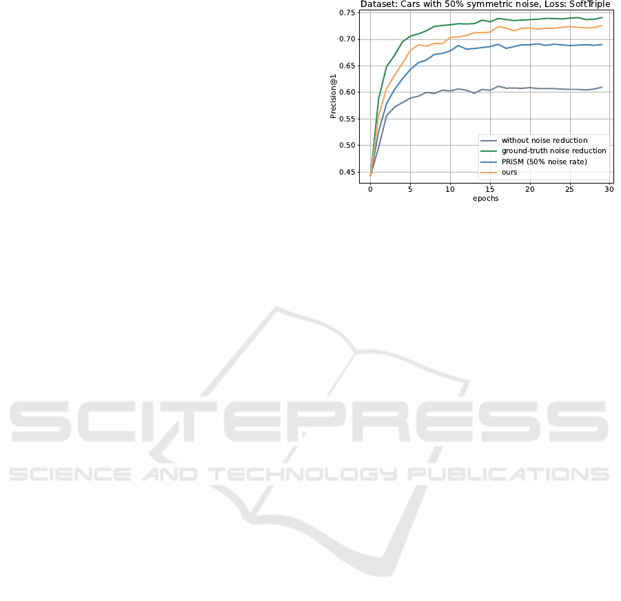
Precision over Training Epochs. Figure 4 reports a
detailed comparison of the effect of predicting and ex-
cluding noisy samples as the model is being trained.
The particular comparison is run on the Cars dataset
with 50% symmetric noise and the SoftTriple loss.
For each of the evaluated methods, we report P@1 on
the test dataset. We observe that the impact of noise
removal is crucial even in the first epochs, those that
establish the good performance of the model in the
later epochs.
4.5 Hyperparameter k
We experimented with hyperparameter k of the near-
est neighbors algorithm. More specifically, we eval-
uated our method using the Cars dataset, 50% sym-
metric noise rate and the SoftTriple loss function. We
did an “offline” evaluation as follows. We first run an
experiment with the above settings using the ground-
truth noise removal approach and stored the features
per epoch. Afterwards, we run our methodology of-
fline, using subsequent epochs as reference and cur-
rent, as it would be encountered in the online ex-
periment, e.g. KNN trained on features of 0th and
noise measured for batches of 1st epoch. We repeated
Figure 4: P@1 over training epochs for the compared meth-
ods.
the same experiment for the different parameteriza-
tion of the nearest neighbors algorithm and evaluated
using the F1-score of the classification of a sample to
noisy vs clean. We chose an offline approach such
that all possible options are evaluated using the ex-
act same set of features rather than features that are
affected due to the model update as guided by noise
removal. Figure 5 shows the results. Very low values,
e.g. k = 1 − 5, were evaluated only for completeness
as they were not expected to capture enough informa-
tion about the neighborhood. We observe that values
around 50 and 400 provide similar high F1-score. We
chose k = 200 which resulted to top average F1-score,
for all the formal experiments and all datasets.
An observation that can be drawn from the re-
sults is that a relatively low k = 20 does not perform
well during initial epochs (F1-score: 76.6%), however
reaches similar F1-score to a much higher k = 1000
during the final epochs. An explanation is that larger
values of k compensate for the fuzzy embedding space
that is encountered during the first epochs, where sim-
ilar samples are not close enough, yet. With this in
mind, one could think the possibility of a variable k,
which lowers as the model stabilizes. Another ap-
proach could be to combine the scores obtained from
different k values such that the noise reduction model
observes both the local and the global neighborhood.
5 CONCLUSIONS
In this work we proposed a simple yet effective ap-
proach to cope with noisy samples during training of
deep metric models. The approach is based on in-
spection of the neighborhood of the samples using
the KNN algorithm and appropriate classification of
samples as noisy according to the presence of sam-
ples that are of the same class as the examined one.
VISAPP 2024 - 19th International Conference on Computer Vision Theory and Applications
602

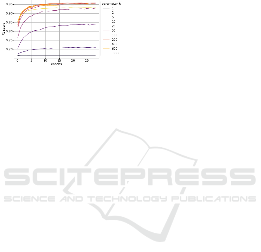
Figure 5: Evaluation of the classification performance of
samples to noisy vs clean using variable k. The reported
metric is the F1-score.
Our approach can be easily plugged in every training
pipeline as a preceding step before loss computation
and possibly triplet mining, without e.g. requiring ar-
chitectural changes and complex schemes. The evalu-
ation in a range of experimental settings demonstrated
that our approach performed better or on par with the
competition, even without the hard requirement about
knowing the noise rate of the dataset.
In future work we will examine more modern
model architectures and other types of noise. We
will also examine re-labeling approaches such that we
can avail from all existing samples without neglecting
them and possibly noise elimination at the level of the
dataset instead of at the level of the batch.
ACKNOWLEDGEMENTS
This work was implemented under the project Craeft
which received funding from the European Union’s
Horizon Europe research and innovation program un-
der grant agreement No 101094349 and was sup-
ported by the Hellenic Foundation for Research and
Innovation (HFRI) under the “1st Call for H.F.R.I Re-
search Projects to support Faculty members and Re-
searchers and the procurement of high-cost research
equipment”, project I.C.Humans, number 91.
REFERENCES
Cai, B., Xiong, P., and Tian, S. (2023). Center con-
trastive loss for metric learning. arXiv preprint
arXiv:2308.00458.
Clanuwat, T., Bober-Irizar, M., Kitamoto, A., Lamb, A.,
Yamamoto, K., and Ha, D. (2018). Deep learn-
ing for classical japanese literature. arXiv preprint
arXiv:1812.01718.
Deng, J., Guo, J., Liu, T., Gong, M., and Zafeiriou, S. Sub-
center arcface: Boosting face recognition by large-
scale noisy web faces. In ECCV.
Deng, J., Guo, J., Xue, N., and Zafeiriou, S. (2019). Ar-
cface: Additive angular margin loss for deep face
recognition. In CVPR.
Falcon, W. A. (2019). Pytorch lightning. GitHub, 3.
Feng, C., Tzimiropoulos, G., and Patras, I. (2022). Ssr:
An efficient and robust framework for learning with
unknown label noise. In BMVC.
Han, B., Yao, Q., Yu, X., Niu, G., Xu, M., Hu, W., Tsang,
I., and Sugiyama, M. (2018). Co-teaching: Robust
training of deep neural networks with extremely noisy
labels. In NIPS.
Ibrahimi, S., Sors, A., de Rezende, R. S., and Clinchant, S.
(2022). Learning with label noise for image retrieval
by selecting interactions. In WACV.
Johnson, J., Douze, M., and J
´
egou, H. (2019). Billion-scale
similarity search with GPUs. IEEE Transactions on
Big Data, 7(3):535–547.
Krause, J., Stark, M., Deng, J., and Fei-Fei, L. (2013). 3d
object representations for fine-grained categorization.
In ICCVW.
LeCun, Y. and Cortes, C. (2010). MNIST handwritten digit
database.
Lee, K.-H., He, X., Zhang, L., and Yang, L. (2018). Clean-
net: Transfer learning for scalable image classifier
training with label noise. In CVPR.
Liu, C., Yu, H., Li, B., Shen, Z., Gao, Z., Ren, P., Xie, X.,
Cui, L., and Miao, C. (2021). Noise-resistant deep
metric learning with ranking-based instance selection.
In CVPR.
Loshchilov, I. and Hutter, F. (2016). Sgdr: Stochastic
gradient descent with warm restarts. arXiv preprint
arXiv:1608.03983.
Musgrave, K., Belongie, S. J., and Lim, S.-N. (2020a). A
metric learning reality check. In ECCV.
Musgrave, K., Belongie, S. J., and Lim, S.-N. (2020b). Py-
torch metric learning. ArXiv, abs/2008.09164.
Oh Song, H., Xiang, Y., Jegelka, S., and Savarese, S.
(2016). Deep metric learning via lifted structured fea-
ture embedding. In CVPR.
Qian, Q., Shang, L., Sun, B., Hu, J., Li, H., and Jin, R.
(2019). Softtriple loss: Deep metric learning without
triplet sampling. In ICCV.
Wah, C., Branson, S., Welinder, P., Perona, P., and Be-
longie, S. (2011). The caltech-ucsd birds-200-2011
dataset.
Wang, X., Han, X., Huang, W., Dong, D., and Scott, M. R.
(2019). Multi-similarity loss with general pair weight-
ing for deep metric learning. In CVPR.
Wang, X., Zhang, H., Huang, W., and Scott, M. R. (2020).
Cross-batch memory for embedding learning. In
CVPR.
Xia, X., Liu, T., Han, B., Gong, C., Wang, N., Ge, Z., and
Chang, Y. (2020). Robust early-learning: Hindering
the memorization of noisy labels. In ICLR.
Yao, Y., Sun, Z., Zhang, C., Shen, F., Wu, Q., Zhang, J.,
and Tang, Z. (2021). Jo-src: A contrastive approach
for combating noisy labels. In CVPR.
Yu, X., Han, B., Yao, J., Niu, G., Tsang, I., and Sugiyama,
M. (2019). How does disagreement help generaliza-
tion against label corruption? In ICML.
Nearest Neighbor-Based Data Denoising for Deep Metric Learning
603