Multi-Agent Quantum Reinforcement Learning Using Evolutionary

Optimization

Michael K

olle

, Felix Topp

, Thomy Phan

, Philipp Altmann

, Jonas N

ußlein

and Claudia Linnhoff-Popien

Institute of Informatics, LMU Munich, Munich, Germany

Thomas Lord Department of Computer Science, University of Southern California, Los Angeles, U.S.A.

ﬁ

Keywords:

Quantum Reinforcement Learning, Multi-Agent Systems, Evolutionary Optimization.

Abstract:

Multi-Agent Reinforcement Learning is becoming increasingly more important in times of autonomous driv-

ing and other smart industrial applications. Simultaneously a promising new approach to Reinforcement

Learning arises using the inherent properties of quantum mechanics, reducing the trainable parameters of a

model signiﬁcantly. However, gradient-based Multi-Agent Quantum Reinforcement Learning methods of-

ten have to struggle with barren plateaus, holding them back from matching the performance of classical

approaches. We build upon an existing approach for gradient free Quantum Reinforcement Learning and

propose tree approaches with Variational Quantum Circuits for Multi-Agent Reinforcement Learning using

evolutionary optimization. We evaluate our approach in the Coin Game environment and compare them to

classical approaches. We showed that our Variational Quantum Circuit approaches perform signiﬁcantly bet-

ter compared to a neural network with a similar amount of trainable parameters. Compared to the larger neural

network, our approaches archive similar results using 97.88% less parameters.

1 INTRODUCTION

Artiﬁcial intelligence (AI) continues to advance,

offering innovative solutions across various do-

mains. Key applications include autonomous driving

(Shalev-Shwartz et al., 2016), the internet of things

(Deng et al., 2020), and smart grids (Dimeas and

Hatziargyriou, 2010). Central to these applications

is the use of Multi-Agent Systems (MAS). These

agents, though designed to act in their own interest,

can be guided to work together using Multi-Agent Re-

inforcement Learning (MARL). Notably, MARL has

proven effective, especially in resolving social dilem-

mas (Leibo et al., 2017b).

Reinforcement Learning (RL) itself has made

impressive strides, outperforming humans in areas

like video games (Badia et al., 2020; Schrittwieser

et al., 2019). Alongside this, quantum technologies

are emerging, suggesting faster problem-solving and

more efﬁcient training in RL (Harrow and Montanaro,

2017). However, Quantum Reinforcement Learning

(QRL) has it’s challenges, such as instabilities and

vanishing gradients (Franz et al., 2022; Chen et al.,

2022). To address these, researchers have turned to

evolutionary optimization methods, as proposed by

(Chen et al., 2022), which have shown promising re-

sults. With the rising prominence of MARL, combin-

ing it with quantum techniques has become a research

focal point, leading to the development of Multi-

Agent Quantum Reinforcement Learning (MAQRL).

In this work, each agent is represented as a Variational

Quantum Circuits (VQC). We employ a evolutionary

algorithm to optimize the parameters of the circuit.

We evaluate different generational evolution strate-

gies and conduct a small scale hyperparameter search

for key parameters of the VQC. Our aim is to evaluate

MAQRL’s capabilities and compare it to traditional

RL methods, using the Coin Game as a benchmark.

In this study, we model each agent using Vari-

ational Quantum Circuits (VQC), a promising and

adaptable representation in the quantum domain. The

inherent ﬂexibility of VQCs allows for the encod-

ing of complex information, making them suitable

for representing agent behaviors in diverse environ-

ments. To ﬁne-tune these quantum circuits and ensure

their optimal performance, we harness the power of

an evolutionary algorithm. This algorithm iteratively

optimizes the parameters of the VQC, guiding the cir-

cuit towards improved decision-making and interac-

tions. While evolutionary algorithms have been tra-

Kölle, M., Topp, F., Phan, T., Altmann, P., Nüßlein, J. and Linnhoff-Popien, C.

Multi-Agent Quantum Reinforcement Learning Using Evolutionary Optimization.

DOI: 10.5220/0012382800003636

Paper published under CC license (CC BY-NC-ND 4.0)

In Proceedings of the 16th International Conference on Agents and Artiﬁcial Intelligence (ICAART 2024) - Volume 1, pages 71-82

ISBN: 978-989-758-680-4; ISSN: 2184-433X

ditionally employed in classical domains, their appli-

cation in the quantum realm offers exciting prospects

for efﬁciently navigating the vast parameter space of

VQCs. As part of our experiements, we systemati-

cally evaluate multiple generational evolution strate-

gies. By comparing their effectiveness, we aim to

identify which strategies most beneﬁcially inﬂuence

the learning trajectories of the VQCs. Furthermore,

recognizing the signiﬁcance of the VQC’s parame-

ters in determining its behavior and effectiveness, we

undertake a small scale hyperparameter search. This

search is dedicated to ﬁne-tuning key parameters, en-

suring the VQC. Central to our research objectives is

the evaluation of MAQRL and its potential contribu-

tions to the ﬁeld. We are particularly interested in

benchmarking MAQRL against established RL tech-

niques to learn its advantages and areas of improve-

ment. For a robust and fair assessment, we have cho-

sen the Coin Game, a well-regarded environment in

multi-agent research, as our testing ground. In sum-

mary our contributions are:

1. Introducting evolutionary optimization in a quan-

tum multi-agent reinforcement learning setting.

2. Assessing the impact of three different genera-

tional evolution strategies and variational layer

counts.

3. Direct comparison to classical approaches with

different parameter counts.

We start in Section 2 by explaining the basics of

MARL and Evolutionary Optimization. We also

give a short introduction to Quantum Computing and

VQCs, and mention related studies (Section 3). Af-

ter outlining our methodology (Section 4) and experi-

mental setup (Section 5), we share the results and im-

plications of our experiments in Section 6. We end

with a summary and thoughts on next steps for re-

search (Section 7). All code and experiments can be

found here

2 PRELIMINARIES

2.1 Multi-Agent Setting

We focus on Markov games M = ⟨D, S, A, P , R ⟩,

where D = {1, ..., N} is a set of agents i, S is a set of

states s

at time step t, A = ⟨A

, ..., A

⟩ is the set of

joint actions a

= ⟨a

t,i

⟩

i∈D

, P (s

t+1

, a

) is the tran-

sition probability, and ⟨r

t,1

, ..., r

t,N

⟩ = R (s

, a

) ∈ R

is the joint reward. π

t,i

) is the action selec-

https://github.com/michaelkoelle/qmarl-evo

tion probability represented by the individual policy

of agent i.

Policy π

is usually evaluated with a value func-

tion V

) = E

t,i

] for all s

∈ S , where G

t,i

∑

∞

k=0

t+k,i

is the individual and discounted return

of agent i ∈ D with discount factor γ ∈ [0, 1) and

π = ⟨π

, ..., π

⟩ is the joint policy of the MAS. The

goal of agent i is to ﬁnd a best response π

∗

with

∗

= max

⟨π

,π

−i

⟩

for all s

∈ S, where π

−i

is the

joint policy without agent i.

We deﬁne the efﬁciency of a MAS or utilitarian

metric (U) by the sum of all individual rewards until

time step T :

U =

∑

i∈D

(1)

where R

∑

T −1

t=0

t,i

is the undiscounted return or sum

of rewards of agent i starting from start state s

2.2 Multi-Agent Reinforcement

Learning

We focus on independent learning, where each agent

i optimizes its individual policy π

based on indi-

vidual information like a

t,i

and r

t,i

using RL tech-

niques, e.g., evolutionary optimization as explained

in Section Evolutionary Optimization. Independent

learning introduces non-stationarity due to simulta-

neously adapting agents which continuously changes

the environment dynamics from an agent’s perspec-

tive ((Littman, 1994; Laurent et al., 2011; Hernandez-

Leal et al., 2017)), which can cause the adoption of

overly greedy and exploitative policies which defect

from any cooperative behavior ((Leibo et al., 2017a;

Foerster et al., 2018)).

2.3 Evolutionary Optimization

Inspired by the process of natural selection, evolution-

ary optimization have been shown to ﬁnd optimal so-

lutions to complex problems, where traditional meth-

ods may not be efﬁcient (Vikhar, 2016). They em-

ploy a population of individuals, randomly generated,

each with its own set of parameters. These individu-

als are evaluated based on a ﬁtness function that mea-

sures how well their parameters perform on the given

problem. The ﬁttest individuals are then selected for

reproduction, where their parameters are recombined

and mutated to form a new population of individuals

for the next generation. (Eiben and Smith, 2015)

Evolutionary optimization approaches like genetic

algorithms (Holland and Miller, 1991) have been used

successfully in a variety of ﬁelds, including the opti-

mization of neural networks, or in interactive recom-

ICAART 2024 - 16th International Conference on Agents and Artiﬁcial Intelligence

mendation tasks (Ding et al., 2011; Gabor and Alt-

mann, 2019). Furthermore these methods have been

used to solve a wide range of problems, from design-

ing quantum circuit architectures to optimizing com-

plex real-world designs (Lukac and Perkowski, 2002;

Caldas and Norford, 2002).

2.4 Quantum Computing

Quantum computing is a emerging ﬁeld of computer

science that uses the principles of quantum mechan-

ics to process information. Similar to classical com-

puters, which store and process data as bits, quantum

computers use quantum bits, or qubits, which can re-

side in multiple states at once (Yanofsky and Man-

nucci, 2008). This property is called superposition.

A state |ψ⟩ of a qubit can generally be expressed as a

linear combination of |0⟩ and |1⟩

|ψ⟩ = α|0⟩+ β|1⟩, (2)

where α and β are complex coefﬁcients that satisfy

the equation

|α|

+ |β|

= 1. (3)

When a qubit in the state of α|0⟩ + β|1⟩ is mea-

sured, its superposition collapses into one of its pos-

sible states, either |0〉 or |1〉, with probabilities deter-

mined by the coefﬁcients |α|

and |β|

respectively

(McMahon, 2007). The quantum system transitions

from a superposition of states to an actual classical

state where the observable’s value is precisely known

(Nielsen and Chuang, 2010). Multiple qubits can

be bound together via entanglement to archive strong

correlations between them.

2.5 Variational Quantum Circuits

VQC, also known as parameterized quantum circuits,

are quantum algorithms that act as function approxi-

mators and are trained using a classical optimization

process. They are commonly used as a drop-in re-

placement for Neural Networks for Deep RL (Chen

et al., 2022; Schuld et al., 2020; Chen and Goan,

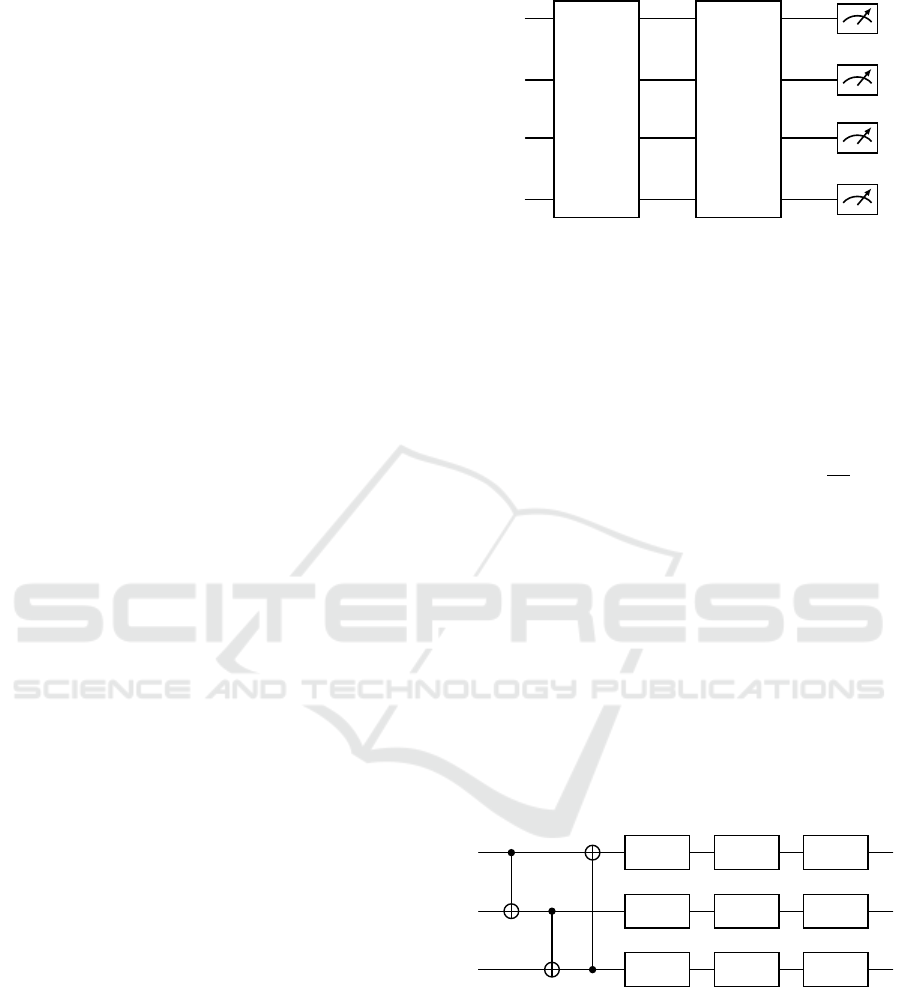
2019; Skolik et al., 2021; Chen, 2022). A VQC is

made up of three stages, as can be seen in Fig. 1. First,

the classical input is embedded into a quantum state in

the State Preperation stage U(x) using superposition.

In the Variational Layers stage V (θ), qubits are then

entangled and parameterized for training. Finally, in

the Measurement stage, the output of the circuit is

measured repeatedly to get the expectation value of

each qubit.

State Preperation. In this work, we use Amplitude

Embedding (Mottonen et al., 2004) to encode classi-

cal data into a quantum state. As the name suggests,

⟩

U(x) V (θ)

⟩

Figure 1: Structure of a Variational Quantum Circuit.

the features are embedded into the amplitudes of

the qubits. Using superposition, we can embed 2

features into n qubits. For Example, if we want to

embed feature vector x ∈ R

in to a 2 qubit quantum

state

⟩

= α

⟩

+ β

⟩

+ γ

⟩

+ δ

⟩

such that

|α|

+ |β|

+ |γ|

+ |δ|

= 1, we ﬁrst pad our feature

vector so that it matches 2

features where n is the

number of qubits used. Next, we normalize the

padded feature vector y such that

∑

−1

k=0

||y||

= 1.

Lastly, we use the state preperation by Mottonen et

al. (Mottonen et al., 2004) to embed the padded and

normalized feature vector into the amplitudes of the

qubit state.

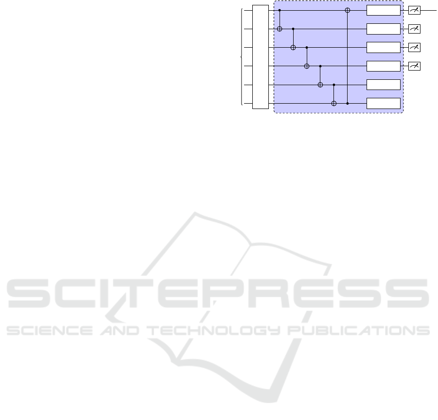
Variational Layers. The second part of the cir-

cuit, referred to as Variational Layers, is made up of

repeated single qubit rotations and entanglers (Fig. 2,

everything within the dashed blue area is repeated L

times, where L is the layer count). We use a layer

architecture inspired by the circuit-centric classiﬁer

design (Schuld et al., 2020) in particular. All of the

circuits presented in this paper employ three single

qubit rotation gates and CNOT gates as entanglers.

RZ(θ

)

RY (θ

) RZ(θ

)

RZ(θ

)

RY (θ

) RZ(θ

)

RZ(θ

)

RY (θ

) RZ(θ

)

θi

denotes a trainable parameter in the circuit

above, where i represents the qubit index and

j ∈ {0, 1, 2} the index of the single qubit rotation

gate. For simplicity, we omitted the index l, which

denotes the current layer in the circuit. The tar-

get bit of the CNOT gate in each layer is given

by(i + l) mod n.

Measurement. The expectation value is mea-

sured in the computational basis (z) of the ﬁrst k

Multi-Agent Quantum Reinforcement Learning Using Evolutionary Optimization

qubits, where k is the dimension of the agents’

actions space. Each measured expectation value is

then given a bias. The biases are also included in the

VQC parameters and are updated accordingly.

3 RELATED WORK

QRL is progressively gaining traction, emanating

from the intersection of RL and the emerging ﬁeld

of QC (Chen et al., 2022; Kwak et al., 2021). This

chapter delves into diverse applications and theoret-

ical concepts within QRL that yield advancements

in parameter reduction, expedited computation times,

and addressing intricate problems.

Initially, we focus on a method by Chen et al.,

wherein parameters are reﬁned using an evolutionary

approach (Chen et al., 2022), forming the foundation

upon which the current work is built. Evolutionary

algorithms have established their efﬁcacy within tra-

ditional RL (Such et al., 2017) and have demonstrated

substantial value for Deep Reinforcement Learning

(DRL). The methodology employed within this re-

search integrates DRL strategies, substituting Neu-

ral Networks with Variational Quantum Circuits as

agents. Chen et al. demonstrated, in a discrete en-

vironment, that VQCs can efﬁciently approximate Q-

value functions in Deep Q-Learning (DQL), present-

ing a quantum perspective to RL, while notably reduc-

ing parameter requirements in comparison to classical

RL. Differing from Chen, the approach presented in

this work incorporates recombination and extends the

gradient free method to the domain of MARL.

An alternative route to Quantum Multi-Agent Re-

inforcement Learning is detailed in (Neumann et al.,

2020; M

uller. et al., 2022) which harnesses Quan-

tum Boltzmann Machines (QBM). The strategy orig-

inates from an extant methodology where QBM out-

performs classical DRL in convergence speed, mea-

sured in the number of requisite time steps, utiliz-

ing Q-value approximation. The outcomes hint at

enhanced stability in learning, and the agents attain-

ing optimal strategies in Grid domains, surmounting

the complexity of the original approach. This method

may serve as a foundational approach in Grid domains

and in other RL domains with superior complexity.

Resemblances to the method employed herein lie in

the utilization of Q-values and grid domains as test-

ing environments.

Moreover, (Yun et al., 2022) explores the appli-

cation of VQCs for QRL and the progression of this

concept to QMARL, bearing similarity to the method-

ology delineated in this thesis. The limited number

of parameters in QRL has demonstrated superior out-

VARIATIONAL LAYER

⟩

U(x)

R(α

, β

, γ

)

R(α

, β

, γ

)

R(α

, β

, γ

)

R(α

, β

, γ

)

R(α

, β

, γ

)

R(α

, β

, γ

)

Figure 2: Variational Quantum Circuit.

comes compared to classical computing. In order to

navigate the challenges of extending this to QMARL

in the Noisy Intermediate-Scale Quantum era and the

non-stationary attributes of classical MARL, a strat-

egy of centralized learning and decentralized execu-

tion is enacted. This approach achieves an overall su-

perior reward in the environments tested, compared

to classical methodologies, with disparities arising in

the employment of evolutionary algorithms and the

architecture of the VQCs.

4 APPROACH

Inspired by to (Chen et al., 2022), we propose to em-

ploy an evolutionary approach to optimize a θ param-

eterized agent. We however consider the more gen-

eral Multi-Agent setup introduced above. Thus, we

aim to optimize the utilitarian metric U (cf. Eq. (1)).

To maximize this ﬁtness function we use a population

P consisting of η random initialized agents, parame-

terized by θ ∈ [−π, π] to match the quantum circuits’

parameter space.

In contrast to previous work, we use VQC rather

than neural networks to approximate the value of the

agent’s actions. This should mainly demonstrate the

improved parameter efﬁciency, as previously denoted,

even applied to complex learning tasks. A VQC con-

sists primarily of three components: the input embed-

ding, the repeated variational layers, and the measure-

ment. Fig. 1 depicts the VQC we employ.

To convert the classical data into a quantum state,

we use Amplitude Embeddings, represented by U(x)

in Fig. 2. Caused by the high dimensionality of most

state spaces, Amplitude Embeddings are currently the

only viable embedding strategy that allow for embed-

ding the whole state information, being able to embed

states in n

qubits.

The second part of the VQCs consists of varia-

tional layers that are variably repeated. Each iteration

increases the number of α

, β

, γ

parameters that are

ICAART 2024 - 16th International Conference on Agents and Artiﬁcial Intelligence

deﬁned by θ and make up each individual to be op-

timized. Per layer, there are n

= n

∗3 parameters,

where n

is the number of qubits. Furthermore, all ro-

tations are performed sequentially as R

(α

), R

(β

)

and R

(γ

). In addition to the parameterized rota-

tions, each variational layer is composed of adjacent

CNOTS to entangle all qubits. After n

repetitions of

the variational layer, the predicted values of the indi-

vidual actions are determined by measuring the ﬁrst

qubits, where n

is the number of actions. This Z-

axis measurement is used to determine the Q-value of

the corresponding action. An agent chooses the action

with the greatest expected value.

The proposed evolutionary algorithm training pro-

cedure to optimize these individuals to maximize the

utilitarian metric U is demonstrated in Algorithm 1.

Data: Population Size η, Number of

Generations µ, Evaluation Steps κ,

Truncation Selection τ, Mutation

Power σ, and Number of Agents N

Result: Population P of optimized agents

← Initialize population η with random θ

for g ∈ {0, 1, ..., µ} do

for i ∈ {0, 1, ..., η} do

Reset testing environment

Score S

t,i

← 0

for t ∈ {0, 1, ..., κ} do

Use policy of agent i for all agents

in env

Select action

← argmax V QC

)

Execute environment step with

action a

Observe reward r

and next state

t+1

t,i

← S

t,i

+ r

end

λ ← Select top τ agents based on S

t,i

Keep top agent based on S

t,i

Recombine η −1 new agents out of λ

Mutate η −1 generated agents

g+1

← η −1 generated agents + top

agent

end

Algorithm 1: Evolutionary optimization algorithm.

For each generation, ﬁrst, the ﬁtness of each indi-

vidual i is evaluated by performing κ steps in the envi-

ronment. Building upon this ﬁtness, the best τ agents

are selected to develop a new generation. In addition,

we employ the so-called elite agent, the agent with

the highest ﬁtness, that is excluded from the follow-

ing mutation procedure.

To form the next generation, mutation and recom-

bination possibilities are combined to generate a new

population. First, new individuals are formed by re-

combining the κ best agents of the current generation

using crossover. The new offspring is produced by

randomly selecting two parents and crossing their pa-

rameters at a randomly selected index. Furthermore,

mutation is applied to generate new agents by modi-

fying the parameters θ of the current generation of the

best τ agents:

θ = θ + σ ∗ε (4)

The agents with the highest ﬁtness values T are the

parents of the upcoming generation. For the mutation,

the parameters θ are modiﬁed as seen in the equa-

tion with the mutation power σ the Gaussian noise

ε ∼ N (′, ∞). Consequently, all θ

parameters undergo

a minor mutation, and new agents, or children, are

generated. Finally, the unaltered elite agent is added

to the child population.

5 EXPERIMENTAL SETUP

5.1 Coin Game Environment

As of today, we are in the Noisy Intermediate-Scale

Quantum era of quantum computing, where we can

simulate only a small number of qubits (Preskill,

2018). This heavily restricts the amount of data we

can embed into the quantum circuit. Therefore, we

are limited in our choices for the evaluation environ-

ment. We chose the Coin Game environment in its

3 ×3 gridworld version due to its relatively small ob-

servation space. The Coin Game, which was created

by (Lerer and Peysakhovich, 2017), is a well-known

sequential game for assessing RL strategies. Both the

Red and Blue agents in the environment are tasked

with collecting coins. Beside the agents there is a sin-

gle coin placed in the grid that corresponds with one

of the agents colors. Fig. 3 depicts a exemplary state

within the Coin Game.

When an agent is in the same position as a coin, it

is deemed collected. After a coin is gathered, a new

coin is generated at a random location, which cannot

be a place occupied by an agent, and is again either

red or blue. A game of the Coin Game is limited to

50 steps 25 per agent, and the objective is to maximize

the agents’ rewards. The Coin Game can be played in

both a competitive and cooperative setting. To make

the game cooperative, the reward for collecting a coin

is increased by +1 for the agent who collects the coin.

Moreover, the second agent’s reward is reduced by -2

if the ﬁrst agent obtains a coin of his color. If we now

consider the agents’ total reward, there is a common

Multi-Agent Quantum Reinforcement Learning Using Evolutionary Optimization

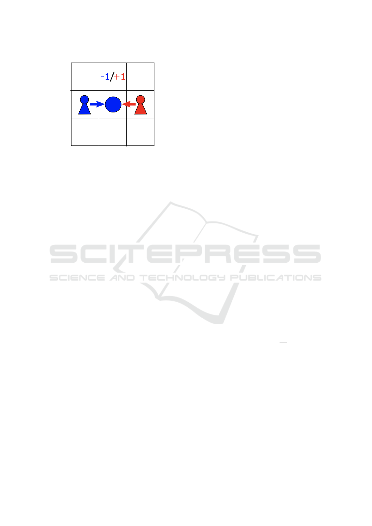
Figure 3: Example State of the Coin Game by (Phan et al.,

2022).

reward of +1 for collecting an own coin and -1 for

collecting an opposing coin. This causes the agents to

be trained to gather their own coins and leave coins,

which are not the agent’s color, for the other agent to

collect. If both agents performed random behaviors,

the expected reward should be zero. As a result of

these rewards, the coin game is a zero-sum game.

Each cell of the 3×3 gridworld can contain either

agent 1, agent 2, a red or blue coin. Empty grids need

not be included in the observation, as movement can

occur on them without consequence at any time. An

agent may select from four possible actions, each of

which is only possible if the ensuing movement does

not lead outside the 3 ×3 gridworld. The numerical

actions range from 0 to 3. Action 0 indicates a step to

the north, action 1 a step to the south, action 2 a step

to the west, and action 3 a step to the east. To prevent

the VQC from choosing illegal actions, the expected

values are normalized to the interval [0, 1] and masked

with environmental regulations.

5.2 Baselines

VQC can be viewed as an alternative to the employ-

ment of classical neural networks as agents. In the

framework of our methodology, we employ neural

networks as agents, as they can be considered gen-

eral approximators. We employ a 2-layer basic neu-

ral network for this purpose. The inputs in the form

of observations are mapped to a variable number x of

hidden units in the ﬁrst layer. The second layer relates

the number of our activities to x hidden units. Hence,

we obtain the individual Q-values for each action, just

as we did with the VQC. Moreover, the Q-values are

multiplied by the action mask to ensure that no ille-

gal action can be selected. Here, we limit ourselves to

this neural network with variable numbers of hidden

units. Similar to the VQC, there are a great number of

ways to alter the network and hence alter the results.

5.3 Metrics

We evaluate our experiments in the Coin Game envi-

ronment using three metrics: Score, Total Coin Rate

and Own Coin Rate. In our work, the agents are

solely playing against themselves, to easily evalu-

ate the agents’ performance. The ﬁrst metric, Score

consists of the undiscounted individual rewards

t,i

until timestep T ∈ {0..49} accumulated over all

agents

∑

i∈{0,1}

T −1

∑

t=0

t,i

(5)

with agent i and generation n ∈{0..99} averaged over

ﬁve seeds. This is a good overall indicator of the

agents performance in the Coin Game environment.

The next two metrics should provide insight into how

the score is reached. The total coins collected metric

is the sum of all collected coins c

t,i

by all agents

until timestep T ∈ {0..49}

∑

i∈{0,1}

T −1

∑

t=0

t,i

(6)

with agent i and generation n ∈{0..99} averaged over

ﬁve seeds. The own coins collected metric OC

the sum of all collected coins that corresponds to the

agents own color o

t,i

until timestep T ∈ {0..49} accu-

mulated over all agents

∑

i∈{0,1}

T −1

∑

t=0

t,i

(7)

with agent i and generation n ∈{0..99} averaged over

ﬁve seeds. Comparing the latter two metrics, we

can get a greater insight how much cooperation is

archived, with the own coin rate OCR:

OCR

∑

i∈{0,1}

T −1

∑

t=0

t,i

(8)

5.4 Training and Hyperparameters

For our experiments in the Coin Game environment,

we train the agents for µ = 100 generations with a

population size of η = 250, pairing the agents against

themselves to play a game of 50 steps 25 per agent.

After a brief preliminary study we set the mutation

power to σ = 0.01. We select the top τ = 5 agents for

regenerating the following population. The VQC has

a Variational Layer count of 4 and n

= 6 qubits to

embed the 36 features of the coin game, resulting in a

parameter count of 76. Each experiment is conducted

with ﬁve different seeds ∈ 0..4 to provide a more

ICAART 2024 - 16th International Conference on Agents and Artiﬁcial Intelligence

accurate indication of performance. Due to current

quantum hardware limitations we use the Pennylane

DefaultQubit simulator for all VQC executions. All

runs were executed on nodes with Intel(R) Core(TM)

i5-4570 CPU @ 3.20GHz.

6 RESULTS

In this section, we present the results of our exper-

iments in the Coin Game environment. We tested

our approach with recombination and mutation com-

bined, as well as mutation only. Furthermore, we

tested two classical neural networks with two hid-

den layers, one with a hidden layer size of 64 ×64

and one with 3 ×4 respectively. The latter conﬁgu-

ration closely matches the amount of parameters that

the VQCs approaches use, to get better insights on the

model-size/performance ratio. Finally, we ran tests

with agents that take random actions at every step

which forms our random baseline. The number of pa-

rameters is listed alongside each approach.

0 25 50 75 100 125 150 175 200

Generation

Average score

VQC(148): Mu

VQC(148): LaReMu

VQC(148): RaReMu

Figure 4: Average Score over the entire population. Each

individual has completed 50 steps in the Coin Game envi-

ronment each generation.

6.1 Comparing Generational Evolution

Strategies

We aim to understand the impact of different gen-

erational evolution strategies. In this section, we

contrast the performance of a mutation-only strat-

egy (Mu) against two combined strategies of mu-

tation and recombination. The ﬁrst combined ap-

proach involves a crossover recombination strategy

at a randomly chosen point in the parameter vec-

tor (RaReMu), while the second employs a layer-

wise crossover (LaReMu). Here, we choose a random

layer and apply the crossover after the last parameter

of the selected layer in the parameter vector. For all

strategies, the mutation power σ is ﬁxed at 0.01.

Examining the average scores depicted in Fig. 4,

the mutation-only strategy emerges as the best

strategy. The crossover strategies showcase simi-

lar performance, though the layerwise method fre-

quently achieves marginally superior outcomes. The

mutation-only strategy starts with an average reward

of 5, dips slightly below 4 by the 17th generation, and

then steadily rises until the 140th generation. From

this point, it ﬂuctuates around a score of 7. In contrast,

the layerwise recombination begins at a lower 3.3, ex-

periences a rapid ascent until the 30th generation, then

stabilizes, eventually reaching an average reward of

6 by the 123rd generation. This is followed by pro-

nounced ﬂuctuations around this value. The random

crossover strategy starts close to the mutation-only at

4.7, but quickly descends to 3 by the 17th genera-

tion. It then steadily climbs until the 131st generation,

achieving a score of 6. However, this score is not sus-

tained and eventually settles around 5.5, making it the

least effective of the three methods.

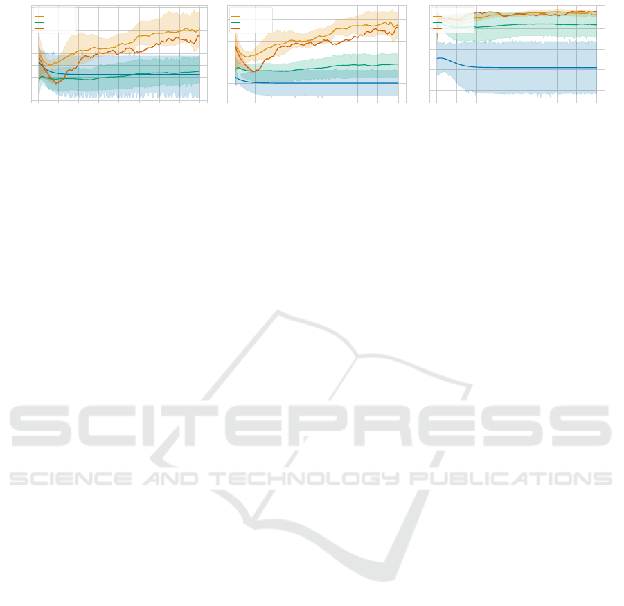
Beyond score comparison, we evaluated the av-

erage number of coins collected during the experi-

ments. As inferred from the scores, the mutation-only

strategy consistently collects more coins, as shown in

Fig. 5a. Although there are periods where the strate-

gies yield almost identical coin counts, at other times,

a gap of up to 2 coins is evident. On average, the com-

bined strategies lag slightly behind the mutation-only

in terms of coin collection.

The layerwise crossover’s initial surge in Fig. 4

correlates with the uptrend in collected coins shown

in Fig. 5a and the coin rate detailed in Fig. 5c.

When comparing the strategies based on these met-

rics, mutation-only consistently achieves the highest

coin rate over all generations and collects the most

coins, accounting for its superior average reward.

The random crossover strategy, while collecting more

coins than the layerwise approach, has a signiﬁcantly

reduced coin rate, resulting in diminished overall re-

wards.

Exploring the coin rate, depicted in Fig. 5c, the

layerwise strategy leads until the 90th generation. Af-

ter that, its rate declines, while the mutation-only

strategy exhibits a gradual, consistent rise. A higher

coin rate indicates enhanced agent cooperation within

the testing environment. This coin rate, combined

with the number of coins collected, determines an

agent’s reward.

In summary, the mutation-only strategy outper-

forms the combined strategies in our experiments. It

not only garners the highest reward but also aligns

best with our objective: maximizing reward. Hence,

subsequent experiments will exclusively employ the

mutation-only approach for the VQCs.

Multi-Agent Quantum Reinforcement Learning Using Evolutionary Optimization

0 25 50 75 100 125 150 175 200

Generation

Average collected coins

VQC(148): Mu

VQC(148): LaReMu

VQC(148): RaReMu

(a) Total coins collected

0 25 50 75 100 125 150 175 200

Generation

Average collected own coins

VQC(148): Mu

VQC(148): LaReMu

VQC(148): RaReMu

(b) Own coins collected

0 25 50 75 100 125 150 175 200

Generation

0.60

0.65

0.70

0.75

0.80

0.85

0.90

0.95

1.00

Own coin rate

VQC(148): Mu

VQC(148): LaReMu

VQC(148): RaReMu

Figure 5: Comparison of (a) average coins collected, (b) average own coins collected and the own coin rate (c) in a 50 step

Coin Game each generation, averaged over 10 seeds.

0 25 50 75 100 125 150 175 200

Generation

Average score

VQC(76)

VQC(112)

VQC(148)

VQC(292)

Figure 6: Average Score over the entire population. Each

individual has completed 50 steps in the Coin Game envi-

ronment each generation.

6.2 Assessing Varying Layer Counts

We investigate the performance dynamics of VQCs

with different layer counts, speciﬁcally with 4, 6,

8, and 16 layers. The relationship between layer

counts and parameters is governed by the formula

3 ∗n ∗6 + 4, where n stands for the number of layers.

Accordingly, VQCs with 4, 6, 8, and 16 layers utilize

76, 112, 148, and 292 parameters respectively. We

trained all VQCs using the mutation-only approach,

setting the mutation strength to σ = 0.01.

Inspecting the average rewards in Fig. 6, all

VQCs, bar the 4-layered one which starts slightly be-

low 3, commence with scores ranging from 5 to 5.5.

By the 25th generation, each VQC stabilizes around

a reward of 4. The 4-layer VQC then gradually as-

cends, consistently holding an average reward of 5

from the 175th generation. The 6-layer VQC ex-

hibits a steady rise until the 62nd generation, with a

more pronounced increase after that, peaking at 6.7

around the 165th generation and subsequently oscil-

lating around 6.5. The 8-layer VQC consistently out-

performs the others, reaching a reward of 5.5 by the

70th generation, encountering a brief plateau, and

then climbing to 7 by the 140th generation. The

16-layer VQC, meanwhile, showcases a pronounced

growth phase between the 25th and 70th generations,

stabilizing around 6 before another rise to 6.5 around

the 160th generation.

For a comprehensive understanding, we next

probe the average coin collection in Fig. 7a. The 4-

layer VQC consistently tops the coin collection met-

ric, progressing from just below 7 to 8. The 6-layer

VQC commences at 6.5, dips to 5.2 by the 23rd gener-

ation, and then rises to 8 by the 165th generation. The

8-layer VQC, despite securing the highest average re-

ward, begins at 6 and only stabilizes around 8 after

the 180th generation. The 16-layer VQC, after an ini-

tial dip, witnesses a rapid increase from the 24th to

103rd generation, brieﬂy declines, and then ﬂuctuates

around 8 coins. Towards the concluding generations,

VQCs with more than 4 layers converge to collect ap-

proximately 8 coins.

Analyzing the own coin count in Fig. 7b, we ob-

serve that, except for the 4-layer VQC, all VQCs ini-

tially decline before ascending. The 4-layer VQC

displays a steady yet modest climb, concluding at a

count of 6.5. The 6-layer VQC takes the longest to

commence its ascent, eventually oscillating around a

count of 7.2. The 8-layer VQC initiates its climb ear-

lier, achieving a slightly higher count of 7.5 by the

end. The 16-layer VQC, notable for its r

Iapid early

ascent, consistently hovers around a count of 7 after

the 100th generation. Among the VQCs, the 4-layer

variant lags, collecting over one own coin fewer than

its counterparts.

Focusing on the own coin rate, the 4-layer VQC

performs the worst. The performance parallels be-

tween the 6-layer and 16-layer VQCs are evident,

both in terms of own coin rate and overall reward.

The standout remains the 8-layer VQC, which, with

its superior own coin rate and comparable coin count,

has the highest reward.

In conclusion, our tests spotlight the 8-layer VQC

as the top performer. Consequently, we select it com-

bined with the the optimal evolutionary strategy out-

lined in 6.1, for all further experiments. This section

underscores that a higher layer count doesn’t guar-

antee superior performance – the 16-layer VQC falls

short of the 8-layer VQC’s achievements. The exper-

ICAART 2024 - 16th International Conference on Agents and Artiﬁcial Intelligence

0 25 50 75 100 125 150 175 200

Generation

Average collected coins

VQC(76)

VQC(112)

VQC(148)

VQC(292)

(a) Total coins collected

0 25 50 75 100 125 150 175 200

Generation

Average collected own coins

VQC(76)

VQC(112)

VQC(148)

VQC(292)

(b) Own coins collected

0 25 50 75 100 125 150 175 200

Generation

0.65

0.70

0.75

0.80

0.85

0.90

0.95

1.00

Own coin rate

VQC(76)

VQC(112)

VQC(148)

VQC(292)

Figure 7: Comparison of (a) average coins collected, (b) average own coins collected and the own coin rate (c) in a 50 step

Coin Game each generation, averaged over 10 seeds.

iments, however, don’t conclusively establish the per-

formance dynamics beyond 200 generations.

0 25 50 75 100 125 150 175 200

Generation

−2

Average score

Random

VQC(148): Mu

NN(147): Mu

NN(6788): Mu

Figure 8: Average Score over the entire population. Each

individual has completed 50 steps in the Coin Game envi-

ronment each generation.

6.3 Comparing Quantum and Classical

Approaches

6.3.1 Comparing VQC and Random

First, we compare the results of our VQC approaches

to the results of the random baseline. In Fig. 8, the

score for the random acting agents is approximately 0,

since the cooperative sequential coin game is a zero-

sum game. The evolutionary-trained VQC approache,

however, perform signiﬁcantly better leading to an av-

erage score around 7. The total coins collected de-

picted in Fig. 9a suggests that in contrast to the ran-

dom agents, the VQC agents successfully learn to col-

lect coins. The own coins collected correlates with

number of collected coins (Fig. 9b). In Fig. 9c we can

see that in neither case the cooperation increases over

time. In summary, trained agents performed signif-

icantly better than random on all metrics, indicating

that the training was successful.

6.3.2 Comparing VQC and Small NN

As depicted in Fig. 8, a better result is achieved by the

VQC approach compared to random. On this basis,

we compare the performance of this VQC approach

to that of a neural network with a comparable number

of parameters. Here we exploit the higher expressive

power of VQCs compared to conventional neural net-

works (Chen et al., 2022). Similar to (Chen et al.,

2022), we deﬁne the expressive power as the capac-

ity to represent particular functions with a constrained

number of parameters. Note that the VQC has 148 pa-

rameters (3 * 6 * 8 + 4). The neural network uses two

hidden layers with dimension 3 and 4 respectively, re-

sulting in a parameter count of 147. Both the neural

network and the VQC, are trained with mutation only

with mutation power σ = 0.01. In Fig. 8, we can see

that the neural network reward ﬂuctuates in the range

of 2.5 to 3. As previously discussed in the last sec-

tion, the VQC approach exhibits a slow learning curve

leading to a signiﬁcant higher score therefore conse-

quently outperforming this neural network. The infe-

rior performance can be explained by the small num-

ber of hidden units and parameters present in neural

networks. Typically, the number of hidden units is

chosen much higher. Further evidence of the neural

network’s deﬁciency is provided by the average num-

ber of coins collected. As shown in Fig. 9a, the NN’s

number of collected coins is below the average score

of the random agents until generation 115 and after

that slightly over it. In comparison, the VQC with

the same number of parameters collects two times as

many coins on average. The neural network is able

to outperform random agents on the basis of its col-

lected own coins, what can be seen in Fig. 9b, lead-

ing to the better performance regarding the own coin

rate (Fig. 9c). In terms of collected own coins and

the own coin rate, the neural network performs sig-

niﬁcantly worse than the VQC with nearly the same

number of parameters. A neural network with this

few hidden units and, consequently, parameters is not

able learn in the coin game environment successfully.

This demonstrates the power of VQCs for RL archiv-

ing signiﬁcantly higher with the same amount of pa-

rameters.

Multi-Agent Quantum Reinforcement Learning Using Evolutionary Optimization

0 25 50 75 100 125 150 175 200

Generation

Average collected coins

Random

VQC(148): Mu

NN(147): Mu

NN(6788): Mu

(a) Total coins collected

0 25 50 75 100 125 150 175 200

Generation

Average collected own coins

Random

VQC(148): Mu

NN(147): Mu

NN(6788): Mu

(b) Own coins collected

0 25 50 75 100 125 150 175 200

Generation

0.2

0.4

0.6

0.8

1.0

Own coin rate

Random

VQC(148): Mu

NN(147): Mu

NN(6788): Mu

Figure 9: Comparison of (a) average coins collected, (b) average own coins collected and the own coin rate (c) in a 50 step

Coin Game each generation, averaged over 10 seeds.

6.3.3 Comparing VQC and Big NN

In the previous section, we observed that a neural

network with the same number of parameters as the

VQC of our approach cannot match the VQC’s per-

formance. We will now compare the results with a

neural network that has signiﬁcantly more parame-

ters. Again, mutation only is used for the evolution

of subsequent generations in both cases and the mu-

tation power is σ = 0.01. We chose a fully connected

NN with two hidden layers of size 64, resulting in

a parameter count of 6788. If we ﬁrst examine the

reward of the neural network and the VQC, we can

see in Fig. 8 that both produce very similar results

over time. Initially, the VQC has a slightly higher

score. From generation 50 onward, there are only

minor differences in terms of average score. Over-

all, the two strategies yield a score of approximatly

7. On the basis of our experiments, we can say that

the VQC achieves nearly identical performance in the

Coin Game environment compared to a neural net-

work that has 46 times more parameters. In Fig. 9a,

the initial value of the VQC method is again higher

than that of the neural network. Due to a steeper

learning curve, the neural network is able to com-

pensate the lower starting value and achieves only

a slightly smaller number of collected coins. From

there are no discernible differences between the two

models. A similar performance of the two approaches

can be seen in Fig. 9b, where the average number

of own coins collected is shown. In Terms of own

coin rate, at ﬁrst, the VQC archives a slightly higher

score. However, at Generation 25, the neural network

initially achieves a better own coin rate before being

slightly lower between Generation 80 and 162. In the

end, the neural network is slightly better in terms of

the own coin rate.

In summary, there is little difference between the out-

comes of the two approaches, despite the neural net-

work having 46 times the number of parameters com-

pared to the VQC. Thus, we can reduce the number

of parameters in our experiments by 97.88% without

sacriﬁcing performance using VQCs. Similar to re-

sults in (Chen et al., 2022), the VQC exhibits a great

expressive power in and we recommend it for future

use in QRL.

7 CONCLUSION

Gradient-based training methods are, as of time of

writing, not suitable for MAQRL due to problems

with barren plateaus and vanishing gradients (Franz

et al., 2022; Chen et al., 2022). In this work, we pre-

sented a alternative approach to gradient based train-

ing methods for MAQRL. We build our approach

upon the evolutionary optimization process used by

(Chen et al., 2022), expanding it to Multi-Agent sys-

tems and different generational evolution strategies.

We proposed three quantum approaches for MARL.

All approaches use VQCs as replacement for neural

networks. Two approach use recombination in addi-

tion to mutation and the third approach mutation only.

For evaluation, we chose Coin Game as our testing

environment due to it’s cooperative setting and rela-

tively small observation space. As baselines, we used

random agents and classical agents with neural net-

works, which were also trained using the evolutionary

algorithm. To achieve a fair comparison, we chose a

neural network with a similar amount of parameters,

as well as one with a hidden layer size of 64 ×64.

In our experiments, we showed that our VQC ap-

proach performs signiﬁcantly better compared to a

neural network with a similar amount of trainable pa-

rameters. Compared to the larger neural network, we

can see that the VQC approach achieves similar re-

sults, showing the effectiveness of using VQCs in a

MAQRL environment. We can reduce the number of

parameters by 97.88% using the VQC approach com-

pared to the similarly good neural network. In com-

parison to previous works (Chen et al., 2022), we used

recombination in addition to mutation in our evolu-

tionary algorithm, which performed worse than muta-

tion alone in the tested setting. Additionally, we used

ICAART 2024 - 16th International Conference on Agents and Artiﬁcial Intelligence

more layers for the VQCs than previous works (Chen

et al., 2022), as they have yielded better results in the

experiments.

In the future, the VQC results could be run not

only on a quantum simulator, but on real quantum

hardware to determine which and if there is a differ-

ence. Also, a comparison of the VQC approach with a

gradient based neural network would be an option for

future work. Another option would be to compare the

VQC approach in terms of the number of parameters

with a data reuploading method and see if this can

solve the coin game similarly well with even fewer

qubits. Additionally, we could work on the hyperpa-

rameters and see if even better results can be achieved

by adapting them.

ACKNOWLEDGEMENTS

This work is part of the Munich Quantum Valley,

which is supported by the Bavarian state government

with funds from the Hightech Agenda Bayern Plus.

REFERENCES

Badia, A. P., Piot, B., Kapturowski, S., Sprechmann, P.,

Vitvitskyi, A., Guo, Z. D., and Blundell, C. (2020).

Agent57: Outperforming the atari human benchmark.

CoRR, abs/2003.13350.

Caldas, L. G. and Norford, L. K. (2002). A design optimiza-

tion tool based on a genetic algorithm. Automation in

construction, 11(2):173–184.

Chen, S. Y. and Goan, H. (2019). Variational quantum

circuits and deep reinforcement learning. CoRR,

abs/1907.00397.

Chen, S. Y.-C. (2022). Quantum deep recurrent reinforce-

ment learning.

Chen, S. Y.-C., Huang, C.-M., Hsing, C.-W., Goan, H.-S.,

and Kao, Y.-J. (2022). Variational quantum reinforce-

ment learning via evolutionary optimization. Machine

Learning: Science and Technology, 3(1):015025.

Deng, S., Xiang, Z., Zhao, P., Taheri, J., Gao, H., Yin, J.,

and Zomaya, A. Y. (2020). Dynamical resource allo-

cation in edge for trustable internet-of-things systems:

A reinforcement learning method. IEEE Transactions

on Industrial Informatics, 16(9):6103–6113.

Dimeas, A. L. and Hatziargyriou, N. D. (2010). Multi-agent

reinforcement learning for microgrids. In IEEE PES

General Meeting, pages 1–8.

Ding, S., Su, C., and Yu, J. (2011). An optimizing bp neural

network algorithm based on genetic algorithm. Artiﬁ-

cial intelligence review, 36:153–162.

Eiben, A. E. and Smith, J. E. (2015). Introduction to evolu-

tionary computing. Springer.

Foerster, J., Chen, R. Y., Al-Shedivat, M., Whiteson, S.,

Abbeel, P., and Mordatch, I. (2018). Learning with

Opponent-Learning Awareness. In Proceedings of the

17th International Conference on Autonomous Agents

and Multiagent Systems, page 122–130, Richland, SC.

International Foundation for Autonomous Agents and

Multiagent Systems.

Franz, M., Wolf, L., Periyasamy, M., Ufrecht, C., Scherer,

D. D., Plinge, A., Mutschler, C., and Mauerer,

W. (2022). Uncovering instabilities in variational-

quantum deep q-networks. Journal of the Franklin

Institute.

Gabor, T. and Altmann, P. (2019). Benchmarking surrogate-

assisted genetic recommender systems. In Proceed-

ings of the Genetic and Evolutionary Computation

Conference Companion, pages 1568–1575.

Harrow, A. W. and Montanaro, A. (2017). Quantum com-

putational supremacy. Nature, 549(7671):203–209.

Hernandez-Leal, P., Kaisers, M., Baarslag, T., and de Cote,

E. M. (2017). A Survey of Learning in Multiagent

Environments: Dealing with Non-Stationarity. arXiv

preprint arXiv:1707.09183.

Holland, J. H. and Miller, J. H. (1991). Artiﬁcial adaptive

agents in economic theory. The American economic

review, 81(2):365–370.

Kwak, Y., Yun, W. J., Jung, S., Kim, J.-K., and Kim, J.

(2021). Introduction to quantum reinforcement learn-

ing: Theory and pennylane-based implementation.

Laurent, G. J., Matignon, L., Fort-Piat, L., et al. (2011). The

world of independent learners is not markovian. Inter-

national Journal of Knowledge-based and Intelligent

Engineering Systems, 15(1):55–64.

Leibo, J. Z., Zambaldi, V., Lanctot, M., Marecki, J.,

and Graepel, T. (2017a). Multi-Agent Reinforce-

ment Learning in Sequential Social Dilemmas. In

Proceedings of the 16th Conference on Autonomous

Agents and Multiagent Systems, AAMAS ’17, page

464–473, Richland, SC. International Foundation for

Autonomous Agents and Multiagent Systems.

Leibo, J. Z., Zambaldi, V. F., Lanctot, M., Marecki, J.,

and Graepel, T. (2017b). Multi-agent reinforce-

ment learning in sequential social dilemmas. CoRR,

abs/1702.03037.

Lerer, A. and Peysakhovich, A. (2017). Maintain-

ing Cooperation in Complex Social Dilemmas us-

ing Deep Reinforcement Learning. arXiv preprint

arXiv:1707.01068.

Littman, M. L. (1994). Markov Games as a Framework

for Multi-Agent Reinforcement Learning. In Machine

Learning Proceedings 1994, pages 157–163. Morgan

Kaufmann, San Francisco (CA).

Lukac, M. and Perkowski, M. (2002). Evolving quan-

tum circuits using genetic algorithm. In Proceedings

2002 NASA/DoD Conference on Evolvable Hardware,

pages 177–185. IEEE.

McMahon, D. (2007). Quantum computing explained. John

Wiley & Sons.

Mottonen, M., Vartiainen, J. J., Bergholm, V., and Salomaa,

M. M. (2004). Transformation of quantum states using

Multi-Agent Quantum Reinforcement Learning Using Evolutionary Optimization

uniformly controlled rotations. arXiv preprint quant-

ph/0407010.

uller., T., Roch., C., Schmid., K., and Altmann., P.

(2022). Towards multi-agent reinforcement learning

using quantum boltzmann machines. In Proceedings

of the 14th International Conference on Agents and

Artiﬁcial Intelligence - Volume 1: ICAART,, pages

121–130. INSTICC, SciTePress.

Neumann, N. M., de Heer, P. B., Chiscop, I., and Phillip-

son, F. (2020). Multi-agent reinforcement learning us-

ing simulated quantum annealing. In Computational

Science–ICCS 2020: 20th International Conference,

Amsterdam, The Netherlands, June 3–5, 2020, Pro-

ceedings, Part VI 20, pages 562–575. Springer.

Nielsen, M. A. and Chuang, I. L. (2010). Quantum Com-

putation and Quantum Information: 10th Anniversary

Edition. Cambridge University Press.

Phan, T., Sommer, F., Altmann, P., Ritz, F., Belzner, L.,

and Linnhoff-Popien, C. (2022). Emergent coopera-

tion from mutual acknowledgment exchange. In Pro-

ceedings of the 21st International Conference on Au-

tonomous Agents and MultiAgent Systems (AAMAS),

pages 1047–1055. International Foundation for Au-

tonomous Agents and Multiagent Systems.

Preskill, J. (2018). Quantum computing in the nisq era and

beyond. Quantum, 2:79.

Schrittwieser, J., Antonoglou, I., Hubert, T., Simonyan, K.,

Sifre, L., Schmitt, S., Guez, A., Lockhart, E., Hass-

abis, D., Graepel, T., Lillicrap, T. P., and Silver, D.

(2019). Mastering atari, go, chess and shogi by plan-

ning with a learned model. CoRR, abs/1911.08265.

Schuld, M., Bocharov, A., Svore, K. M., and Wiebe, N.

(2020). Circuit-centric quantum classiﬁers. Physical

Review A, 101(3):032308.

Shalev-Shwartz, S., Shammah, S., and Shashua, A. (2016).

Safe, multi-agent, reinforcement learning for au-

tonomous driving. CoRR, abs/1610.03295.

Skolik, A., McClean, J. R., Mohseni, M., van der Smagt, P.,

and Leib, M. (2021). Layerwise learning for quantum

neural networks. Quantum Machine Intelligence, 3:1–

11.

Such, F. P., Madhavan, V., Conti, E., Lehman, J., Stanley,

K. O., and Clune, J. (2017). Deep neuroevolution: Ge-

netic algorithms are a competitive alternative for train-

ing deep neural networks for reinforcement learning.

CoRR, abs/1712.06567.

Vikhar, P. A. (2016). Evolutionary algorithms: A critical

review and its future prospects. In 2016 International

Conference on Global Trends in Signal Processing,

Information Computing and Communication (ICGT-

SPICC), pages 261–265.

Yanofsky, N. S. and Mannucci, M. A. (2008). Quantum

computing for computer scientists. Cambridge Uni-

versity Press.

Yun, W. J., Park, J., and Kim, J. (2022). Quantum multi-

agent meta reinforcement learning.

ICAART 2024 - 16th International Conference on Agents and Artiﬁcial Intelligence